3 Sequences & Series
We have talked about how exponentials can model growth, but in our day to day we don’t always encounter growth in this continuous way as a curve. Rather, we encounter it in a discrete way as a sequence.
3.1 Arithmetic
Say I set myself a New Years resolution of reading more. At the moment I read about 3 pages per night, but I have the idea to increase this by two pages every day in January. On the January 1st I’ll read 5 pages, on Jan 2nd read 7 pages, on Jan 3rd read 9 pages, and so on. The number of pages I will is a sequence: \[ 5, 7, 9, \ldots. \]
The \(n^{\text{th}}\) term in a sequence is denoted \(a_n\), so here \(a_1 = 5\), \(a_2 = 7\), etc. By observation we might be able to see that on the \(n^{\text{th}}\) day I will have read \(3+2n\) pages, so here \(a_n = 3+2n\).
This means that we can work out a given term in the sequence without calculating all the intermediate terms. For example, on January 31st I’ll read \(a_{31} = 3 + 2\times31 = 65\) pages.
In general, We define the \(n^{\text{th}}\) term of an arithmetic sequence as \(a_n = a_0 + nd\), where \(a_0\) is our starting value and \(d\) is the difference we move by each term.
So in the reading previous example, \(a_0 = 3\) and \(d = 2\).
Suppose now I want to find how many pages \(S\) I will read in January total. This would be the \[ S = a_1 + a_2 + \cdots + a_{31}. \] We could compute this by hand, but there exists a handy formula \[ S_n = a_1 + a_2 + \cdots + a_{n} = \frac{n(a_1 + a_n)}{2}. \]
This sum is called an arithmetic series and you may also see this sum denoted using ‘sigma’ notation \[ S_n = \sum_{m=1}^{n} a_m = \frac{n(a_1 + a_n)}{2}. \]
For my reading goal, that means \[ S_{31} = \sum_{n=1}^{31}(3+2n) = \frac{31(5 + 65)}{2} = \frac{31\times70}{2} = 1085. \] That’s almost the same number of pages as War and Peace, so probably not realistic as resolutions go!
3.2 Geometric
Another context where growth comes up is in savings or interest. Say I put \(\text{£}50\) in a savings account with 2% annual interest. That is, at the end of the year 2% of the total balance is added extra by the bank.
At the end of the first year, it will contain \(\text{£}50 + 2\%\times\text{£}50 = \text{£}50 + \text{£}1 = \text{£}51\). Next year though, \(2\%\) of my balance isn’t \(\text{£}1\) any more, it’s \(2\%\times\text{£}51 = \text{£}1.02\).
By remembering that increasing by \(2\%\) is the same as multiply by \(1 + \frac{2}{100} = 1.02\), we can put To put it back in the language of sequences as \[\begin{align*} a_0 &= \text{£}50 \\ a_1 &= \text{£}50 \times 1.02 \\ a_2 &= (\text{£}50 \times 1.02) \times 1.02 \\ a_3 &= ((\text{£}50 \times 1.02) \times 1.02) \times 1.02 \\ \end{align*}\] or, simplifying using powers, \(a_n = \text{£50}\times{1.02}^n\). That means in thirty five years my savings pot will be a whole \[ a_{35} = 50\times1.02^{35} = 99.99448. \] Well, \(\text{£}99.99\) isn’t nothing, but it’s certainly not a retirement fund.
In general, We define the \(n^{\text{th}}\) term of an geometric sequence as \(a_n = a_0 \times r^n\), where \(a_0\) is our starting value and \(r\) is the common ratio we increase by each term.
In the previous example, \(a_0 = 50\) and \(r = 1.02\). Similar to before, we can compute the sum of these terms - the geometric series.
\[ S_n = a_1 + a_2 + \cdots + a_{n} = \frac{a_0(1-r^n)}{1-r}. \] This formula doesn’t hold when \(r = 1\) since it would require dividing by zero, though in that case the value of \(S_n\) can be worked out directly from its definition.
3.2.1 Exponential Growth
Geometric series with \(r > 1\) are often used to model exponential growth. For example, what if \(a_0 = 2\), \(r = 2\) then the initially small numbers will increase initially slowly but faster and faster: \[ 2, 4, 8, 16, 32, 64, 128, \ldots \]
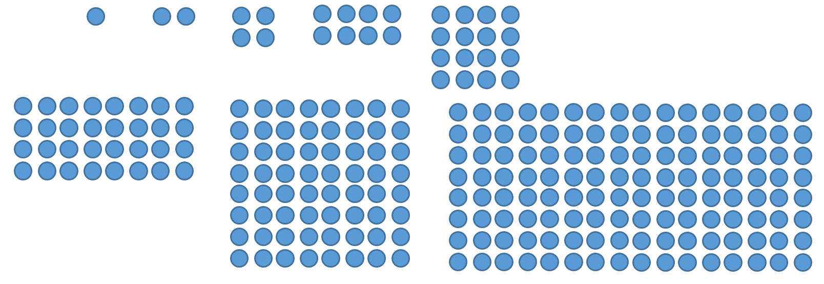
With each step, the increase is twice as large as the previous step.