| Variable Name | Description |
|---|---|
| Name | Name of the institution |
| State | US state where the institution is located |
| ID | Institution ID number |
| Main | Main campus indicator (1 = main campus, 0 = branch campus) |
| Control | Control of institution (Private, Profit, Public) |
| Region | US region (Midwest, Northeast, Southeast, West, etc.) |
| Locale | Locale type (City, Suburb, Town, Rural) |
| Enrollment | Undergraduate enrolment (number of students) |
| AdmitRate | Admission rate (proportion of applicants admitted) |
| Cost | Average total cost (tuition, room, board, etc.) |
| PartTime | Percent of undergraduates who are part-time students |
| TuitionIn | In-state tuition and fees |
| TuitionOut | Out-of-state tuition and fees |
– MSDA IFP
Week 11 – Tutorial 04 Hypothesis Testing & t-test
1. Tasks for formative report
This week’s task is highlighted in bold below. Please only focus on completing that task this week. In the next section, you will also find guided sub-steps you may want to consider to complete this week’s task.
- Read the College dataset into R, inspect it, and write a concise introduction to the data and its structure.
- Display and describe the categorical variables.
- Display and describe a selection of numeric variables.
4) Test at least one research question using an appropriate hypothesis test.
- Finish the report write-up, knit to PDF, and submit.
This tutorial is designed to help you complete Task 4.
1.1 Task 4 – sub-tasks
Tip
Tip: Hover over the footnotes for hints showing useful R functions.
This week you will focus on Task 4: Test at least one research question using an appropriate hypothesis test.
Below are guided sub-steps you may want to follow, using the structure required in Assessment Stage 2.
Your required structure for each research question
For each research question, you must complete these steps in order:
- State the research question in your own words.
- Write the null hypothesis (\(H_0\)) and the alternative hypothesis (\(H_1\)).
- Identify the variables involved and their roles (grouping variable, outcome variable).
- Consider which statistical test is appropriate, and justify your choice.
- Prepare the data only as required to answer the research question
(minimal subsetting only where necessary).
- Conduct the statistical analysis in R.
- Report the relevant statistical output
(t, df, p-value, and confidence interval).
- Produce one appropriate visualisation and refer to it in the text.
Your writing should be clear and concise.
Interpretation should be brief and factual.
Data
CollegeScores Dataset
You will work with the CollegeScores dataset in this tutorial.
At the link CollegeScores_teaching_final.csv you will find information about 400 higher-education institutions in the United States.
The dataset includes variables describing each institution’s location, sector (public/private), tuition costs, enrolment, and the demographic composition of their student body.
Research questions for this tutorial
For Task 4, you must answer the following research questions using an independent-samples t-test.
- Research question 1 (RQ1)
Do Public and Private institutions differ in their average total cost?
- Research question 2 (RQ2)
Do institutions located in Cities differ in their averagenundergraduate enrollment compared to institutions in Rural areas?
- Research question 3 (RQ3)
Do Private institutions have higher average admission rates than Public institutions?
Required structure for each research question
For each research question, you must follow the **full analysis
structure** outlined earlier in this tutorial. Your work must include,
in this order:
a clear statement of the research question,
the null hypothesis ($H_0$) and alternative hypothesis ($H_1$),
identification of the variables involved and their roles,
justification of the choice of statistical test,
any data preparation or subsetting required to answer the question,
the statistical analysis in R,
appropriate reporting of results (t, df, p-value, and
confidence interval), and
a brief, factual interpretation of the results.
Your interpretation should be statistical only and should not make any causal claims.
library(tidyverse)── Attaching core tidyverse packages ──────────────────────── tidyverse 2.0.0 ──
✔ forcats 1.0.1 ✔ readr 2.2.0
✔ ggplot2 4.0.2 ✔ stringr 1.6.0
✔ lubridate 1.9.5 ✔ tidyr 1.3.2
✔ purrr 1.2.1
── Conflicts ────────────────────────────────────────── tidyverse_conflicts() ──
✖ dplyr::filter() masks stats::filter()
✖ dplyr::lag() masks stats::lag()
ℹ Use the conflicted package (<http://conflicted.r-lib.org/>) to force all conflicts to become errorscollege <- read_csv("CollegeScores_teaching.csv")Rows: 400 Columns: 17
── Column specification ────────────────────────────────────────────────────────
Delimiter: ","
chr (5): Name, State, Control, Region, Locale
dbl (12): ID, Main, Enrollment, PartTime, TuitionIn, TuitionOut, White, Blac...
ℹ Use `spec()` to retrieve the full column specification for this data.
ℹ Specify the column types or set `show_col_types = FALSE` to quiet this message.glimpse(college)Rows: 400
Columns: 17
$ ID <dbl> 101189, 101569, 101693, 105534, 106148, 106625, 107220, 107…
$ Name <chr> "Faulkner University", "Lawson State Community College", "U…
$ State <chr> "AL", "AL", "AL", "AZ", "AZ", "AR", "AR", "AR", "AR", "AR",…
$ Main <dbl> 1, 1, 1, 1, 1, 1, 1, 1, 1, 1, 1, 1, 1, 1, 1, 1, 1, 1, 1, 1,…
$ Control <chr> "Private", "Public", "Private", "Profit", "Public", "Public…
$ Region <chr> "Southeast", "Southeast", "Southeast", "West", "West", "Sou…
$ Locale <chr> "City", "City", "Rural", "City", "City", "Rural", "City", "…
$ Enrollment <dbl> 2272, 3034, 1276, 2300, 4682, 1216, 169, 50, 642, 106, 2908…
$ PartTime <dbl> 23.3, 43.1, 9.7, 0.0, 65.1, 27.3, 0.0, 0.0, 42.7, 18.9, 80.…
$ TuitionIn <dbl> 20970, 4440, 22210, 12992, 2280, 3120, 13695, 15825, 3680, …
$ TuitionOut <dbl> 20970, 8010, 22210, 12992, 8976, 5448, 13695, 15825, 6530, …
$ White <dbl> 41.5, 14.9, 61.7, 39.5, 46.2, 93.3, 75.7, 2.0, 70.6, 85.9, …
$ Black <dbl> 49.7, 80.8, 18.6, 6.4, 0.9, 2.6, 7.7, 98.0, 19.5, 2.8, 7.8,…
$ Hispanic <dbl> 2.0, 1.6, 2.1, 39.0, 26.7, 1.9, 11.8, 0.0, 4.5, 8.5, 24.7, …
$ Asian <dbl> 0.4, 0.8, 1.4, 5.2, 0.7, 0.1, 1.8, 0.0, 0.5, 0.9, 10.6, 2.3…
$ Other <dbl> 6.5, 2.0, 16.2, 10.0, 25.6, 2.1, 3.0, 0.0, 5.0, 1.9, 17.3, …
$ AdmitRate <dbl> 0.5101, NA, 0.4702, NA, NA, NA, NA, NA, NA, NA, NA, NA, 0.6…2 Worked example: Independent-samples t-test
In this worked example, we illustrate the full reasoning process behind a hypothesis test, from a research question to statistical analysis and reporting.
The aim is to show how statistical analysis is driven by a research question, not by R commands.
We use the dataset provided in datasets/HollywoodMovies.csv, which contains information on 1295 films, including their genre and audience ratings.
To make this comparison suitable for a statistical test, we will focus on two genres only.
| Variable Name | Description |
|---|---|
| Movie | Title of the movie |
| LeadStudio | Primary U.S. distributor |
| RottenTomatoes | Critics' rating (Rotten Tomatoes) |
| AudienceScore | Audience rating (Rotten Tomatoes) |
| Genre | Film genre (e.g., Action Adventure, Comedy, Thriller) |
| TheatersOpenWeek | Number of screens on opening weekend |
| OpeningWeekend | Opening weekend gross (in millions) |
| BOAvgOpenWeekend | Average box office income per theatre, opening weekend |
| Budget | Production budget (in millions) |
| DomesticGross | U.S. gross income (in millions) |
| ForeignGross | Foreign gross income (in millions) |
| WorldGross | Worldwide gross income (in millions) |
| Profitability | Worldwide gross as a percentage of budget |
| OpenProfit | Percentage of budget recovered on opening weekend |
| Year | Year of release |
These data were compiled from Box Office Mojo, The Numbers, and Rotten Tomatoes.
2.1 Research context and research question
Film researchers and studios are often interested in understanding how different types of films are received by audiences. One question of interest is whether audience ratings differ systematically across film genres.
In this example, we focus on audience ratings and ask whether the average audience score differs between two film genres.
Research question
RQ1: Do Drama and Comedy films differ in their average audience rating?
RQ2: Do Action Adventure films have higher average audience ratings than Comedy films?
RQ1: Do Drama and Comedy films differ in their average audience rating?
2.2 Hypotheses
Hypotheses are always stated in terms of population parameters, not sample statistics.
Let \(\mu_1\) and \(\mu_2\) denote the population mean audience ratings for Drama and Comedy films, respectively.
Null hypothesis (\(H_0\)):
The mean audience rating is the same for the two genres
(\(\mu_1 = \mu_2\)).Alternative hypothesis (\(H_1\)):
The mean audience rating differs between the two genres
(\(\mu_1 \neq \mu_2\)).
Because the alternative hypothesis does not specify a direction, this is a non-directional hypothesis, and we will use a two-sided test.
2.3 Variables and their roles
To answer the research question, we identify the relevant variables:
Grouping variable:
Genre
A categorical variable that defines the two independent groups (Drama and Comedy).Outcome variable:
AudienceScore
A numeric variable whose mean is compared across the two groups.
2.4 Choosing the statistical test
An independent-samples t-test is appropriate because:
- the outcome variable (
AudienceScore) is numeric,
- the grouping variable (
Genre) defines two independent groups, and
- the research question concerns a difference in population means.
2.5 Significance level
Before analysing the data, we choose a significance level.
For this analysis, we set:
\(\alpha\) = 0.05
This means that, if the null hypothesis is true, we are willing to accept a 5% chance of rejecting it incorrectly.
2.6 Data preparation
The variable Genre contains more than two categories. To meet the requirements of an independent-samples t-test, we restrict the dataset to two genres.
movies <- read_csv("HollywoodMovies.csv")Subsetting
movies_ttest <- movies |>
  filter(Genre %in% c("Drama", "Comedy")) |>
  mutate(Genre = factor(Genre))
movies_ttest
# A tibble: 577 × 15
Movie LeadStudio RottenTomatoes AudienceScore Genre TheatersOpenWeek
<chr> <chr> <dbl> <dbl> <fct> <dbl>
1 21 Jump Street Sony Pict… 85 82 Come… 3121
2 A Late Quartet Entertain… 76 71 Drama 9
3 A Royal Affair Magnolia … 90 82 Drama 7
4 Albert Nobbs Roadside … 56 47 Drama 245
5 American Reun… Universal… 44 63 Come… 3192
6 Amour Sony Pict… 93 82 Drama 3
7 Anna Karenina Focus Fea… 63 51 Drama 16
8 Barfi! UTV Motio… 86 86 Come… 132
9 Beasts of the… Fox Searc… 86 76 Drama 4
10 Big Miracle Universal… 74 64 Drama 2129
# ℹ 567 more rows
# ℹ 9 more variables: OpeningWeekend <dbl>, BOAvgOpenWeekend <dbl>,
# Budget <dbl>, DomesticGross <dbl>, WorldGross <dbl>, ForeignGross <dbl>,
# Profitability <dbl>, OpenProfit <dbl>, Year <dbl>Visualising the groups
ggplot(movies_ttest, aes(x = Genre, y = AudienceScore)) +
  stat_summary(
    fun = mean,
    geom = "bar",
    fill = "#A6CEE3",
    colour = "black"
  ) +
  stat_summary(
    fun.data = mean_cl_normal,
    geom = "errorbar",
    width = 0.2
  ) +
  stat_summary(
    fun = mean,
    geom = "text",
    aes(label = round(after_stat(y), 1)),
    vjust = -0.5,
    size = 5
  ) +
  coord_cartesian(ylim = c(0, 100)) +
  labs(
    title = "Mean audience ratings by film genre",
    subtitle = "Error bars show 95% confidence intervals",
    x = "Film genre",
    y = "Mean audience rating"
  ) +
  theme_minimal(base_size = 14)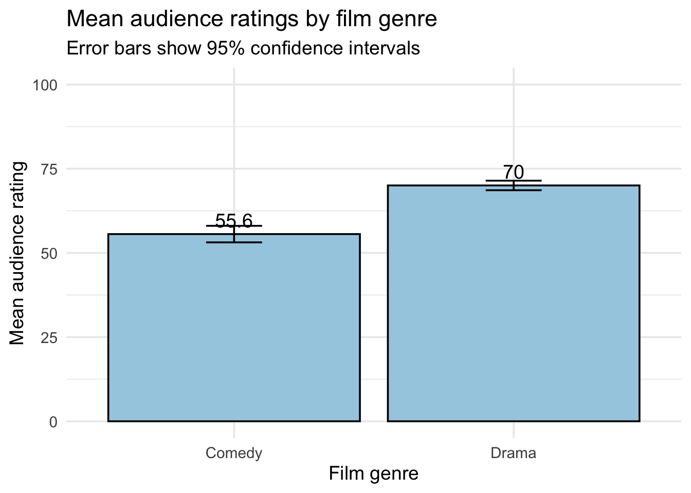
The barplot shows that Drama films have a higher mean audience rating than Comedy films.
now we will test of the difference between the group means is consistent with the result of the t-test.
Code
What does
stat_summary()do?stat_summary()tells R to calculate a summary statistic for each group and then plot it.Instead of plotting every individual data point, we are plotting summaries of the data.
fun = mean→ tells R to calculate the mean ofAudienceScorefor each group (e.g. Comedy, Drama)geom = "bar"→ tells R to draw those means as barsfillandcolour
→ control the appearance of the bars (inside colour and border)
Second part: the error bars (uncertainty)
This part adds error bars on top of the bars.
fun.data = mean_cl_normal→ tells R to calculate:the mean, and
a 95% confidence interval around the mean
geom = "errorbar"→ draws vertical lines showing that intervalwidth = 0.2→ controls how wide the little horizontal caps are
2.7 Conducting the statistical analysis in R
We now conduct the independent-samples t-test to compare the mean audience ratings of Drama and Comedy films.
t_test_movies <- t.test(
  AudienceScore ~ Genre,
  data = movies_ttest
)

t_test_movies
    Welch Two Sample t-test

data:  AudienceScore by Genre
t = -10.035, df = 321.68, p-value < 2.2e-16
alternative hypothesis: true difference in means between group Comedy and group Drama is not equal to 0
95 percent confidence interval:
 -17.27971 -11.61477
sample estimates:
mean in group Comedy  mean in group Drama
            55.59162             70.03886
How to read the t-test output
R reports the results of a hypothesis test in a standard format.
Each part of the output corresponds to something you are expected to report and interpret.
Welch Two Sample t-test
This line tells us which version of the t-test was used.
By default, R uses Welch’s independent-samples t-test, which does not assume equal variances between the two groups.
This is the recommended default and is appropriate for this course.
data: AudienceScore by Genre
This confirms the variables used in the test:
- Outcome variable:
AudienceScore - Grouping variable:
Genre
t = -10.035
This is the test statistic.
- The t value measures how far apart the two sample means are, relative to the variability in the data.
- The negative sign reflects the order of subtraction used by R (Comedy − Drama).
- For a two-sided test, the sign itself is not important.
df = 321.68
This is the degrees of freedom.
- Because Welch’s t-test is used, the degrees of freedom are not necessarily an integer.
- Degrees of freedom indicate how much information the test is based on and must always be reported with the t statistic.
p-value < 2.2e-16
This is the p-value.
- The p-value is far smaller than the chosen significance level (\(\alpha = 0.05\)).
- This means the observed difference would be very unlikely if the null hypothesis were true.
Decision:
Because p < 0.05, we reject the null hypothesis.
Alternative hypothesis
true difference in means between group Comedy and group Drama is not equal to 0
This restates the alternative hypothesis.
- “Not equal to 0” confirms that this is a two-sided test, matching the non-directional hypothesis stated earlier.
95 percent confidence interval
[-17.28, −11.61]
This is the 95% confidence interval for the population mean difference (Comedy − Drama).
- The interval does not include 0, which is consistent with a statistically significant result.
- The entire interval is negative, indicating that Comedy films have lower average audience ratings than Drama films.
Sample estimates
- Mean audience score (Comedy): 55.59
- Mean audience score (Drama): 70.04
These are the sample means for each group.
The hypothesis test evaluates whether this observed difference is likely to reflect a real difference in the population.
Key takeaway
- The p-value tells us whether the difference is unlikely under the null hypothesis.
- The confidence interval tells us which population differences are plausible.
- The degrees of freedom indicate how much information the test is based on.
All three should be reported together.
2.8 Interpretation
The independent-samples t-test showed a statistically significant difference in mean audience ratings between Drama and Comedy films, t(321.68) = −10.04, p < .001. Because the p-value is smaller than the chosen significance level (\(\alpha = 0.05\)), we reject the null hypothesis that the population mean audience ratings are equal for the two genres.
The 95% confidence interval for the mean difference (Comedy − Drama) was [−17.28, −11.61], which does not include 0. This indicates that a true difference in average audience ratings between Drama and Comedy films is plausible in the population.
The sample means suggest that Drama films receive higher average audience ratings (M = 70.04) than Comedy films (M = 55.59). This interpretation is factual, based directly on the statistical output, and does not imply any causal relationship between genre and audience ratings.
RQ2: Do Action Adventure films have higher average audience ratings than Comedy films?
Hypotheses
Let \(\mu_{\text{Action}}\) = population mean audience rating for Action films \(\mu_{\text{Comedy}}\) = population mean audience rating for Comedy films
Null hypothesis (\(H_0\)): \(\mu_{\text{Action}} \le \mu_{\text{Comedy}}\)
Alternative hypothesis (\(H_1\)): \(\mu_{\text{Action}} > \mu_{\text{Comedy}}\)
Because the alternative hypothesis specifies a direction, this is a directional hypothesis, and we use a one-sided test.
2.11 Variables and their roles
Grouping variable: Genre (categorical; Action vs Comedy)
Outcome variable: AudienceScore (numeric; the variable whose mean is compared across groups)
2.12 Choosing the statistical test
An independent-samples t-test is appropriate because:
the outcome variable (AudienceScore) is numeric,
the grouping variable (Genre) defines two independent groups, and
the research question concerns a difference in population means.
The test itself is the same as for RQ1; what changes is the direction specified in the hypothesis.
2.13 Data preparation
To answer this research question, we subset the dataset to include only Action Adventure and Comedy films.
movies_action_comedy <- movies |>
  filter(Genre %in% c("Action", "Comedy")) |>
  mutate(Genre = factor(Genre))

movies_action_comedy
# A tibble: 361 × 15
Movie LeadStudio RottenTomatoes AudienceScore Genre TheatersOpenWeek
<chr> <chr> <dbl> <dbl> <fct> <dbl>
1 21 Jump Street Sony Pict… 85 82 Come… 3121
2 Act of Valor Relativit… 27 72 Acti… 3039
3 Agneepath Eros Inte… 91 62 Acti… 132
4 American Reun… Universal… 44 63 Come… 3192
5 Barfi! UTV Motio… 86 86 Come… 132
6 Battleship Universal… 34 55 Acti… 3690
7 Casa de mi Pa… Lionsgate 41 35 Come… 382
8 Celeste & Jes… Sony Pict… 71 62 Come… 4
9 Contraband Universal… 51 58 Acti… 2863
10 Dabangg 2 Eros Inte… 36 50 Come… 166
# ℹ 351 more rows
# ℹ 9 more variables: OpeningWeekend <dbl>, BOAvgOpenWeekend <dbl>,
# Budget <dbl>, DomesticGross <dbl>, WorldGross <dbl>, ForeignGross <dbl>,
# Profitability <dbl>, OpenProfit <dbl>, Year <dbl>2.15 Conducting the statistical analysis in R
We now conduct an independent-samples t-test with a one-sided alternative hypothesis.
t_test_action_comedy <- t.test(
  AudienceScore ~ Genre,
  data = movies_action_comedy,
  alternative = "greater"
)

t_test_action_comedy
    Welch Two Sample t-test

data:  AudienceScore by Genre
t = 3.1723, df = 351.6, p-value = 0.0008228
alternative hypothesis: true difference in means between group Action and group Comedy is greater than 0
95 percent confidence interval:
 2.805673      Inf
sample estimates:
mean in group Action mean in group Comedy
            61.43529             55.59162
What does
alternative = "greater" mean?
In an independent-samples t-test, the alternative argument specifies which kind of research hypothesis we are testing.
There are three possible options:
alternative = "two.sided"
Tests whether the two population means are different
(no direction specified).alternative = "greater"
Tests whether the mean of the first group is greater than the mean of the second group.alternative = "less"
Tests whether the mean of the first group is less than the mean of the second group.
How does R decide which group comes first?
In a formula like:
AudienceScore ~ GenreIn this dataset:
"Action"comes before"Comedy"
As a result, R computes and tests the difference:
\[ \mu_{\text{Action}} - \mu_{\text{Comedy}} \]
This ordering determines how the t statistic, confidence interval, and alternative hypothesis are defined.
Why do we use alternative = "greater" here?
Our research question is directional:
Do Action films have higher average audience ratings than Comedy films?
This corresponds to the alternative hypothesis:
\[ H_1: \mu_{\text{Action}} > \mu_{\text{Comedy}} \]
Because we are explicitly testing whether the mean audience score for Action films is greater than the mean for Comedy films, we specify:
alternative = "greater"What do the other alternative options mean?
alternative = "two.sided"
Tests whether the two population means are different, without
specifying a direction:\[ H_1: \mu_{\text{Action}} \neq \mu_{\text{Comedy}} \]
alternative = "less"
Tests whether the mean of the first group (Action) is lower than
the mean of the second group (Comedy):\[ H_1: \mu_{\text{Action}} < \mu_{\text{Comedy}} \]
Important rule for this course
The choice of
alternativemust be determined by the research question before looking at the data.Choosing
"greater"or"less"after inspecting the sample means is not valid statistical practice.When no direction is stated in advance, always use a two-sided test.
2.16 Interpretation
The independent-samples t-test with a one-sided alternative hypothesis showed a statistically significant difference in mean audience ratings between Action and Comedy films, t(351.6) = 3.17, p = 0.0008.
Because the p-value is smaller than the chosen significance level (\(\alpha = 0.05\)), we reject the null hypothesis.
The alternative hypothesis stated that Action films have higher average audience ratings than Comedy films. Consistent with the directional alternative hypothesis, Action films received higher average audience ratings than Comedy films. In the sample, the mean audience score for Action films was 61.44, compared to 55.59 for Comedy films, indicating a higher typical audience rating for Action films.
The 95% confidence interval for the mean difference (Action − Comedy) was [2.81, \(\infty\) ), indicating that, in the population, Action films are expected to have audience ratings that are at least about 2.8 points higher than Comedy films.
This interpretation is purely statistical and does not imply any causal relationship between film genre and audience ratings.