scores <- c(8, 9, 11, 12)
scores
[1] 8 9 11 12In statistics, we usually want to learn something about a population, but it is rarely possible to collect data from everyone in that population. Instead, we work with a sample and use it to make informed statements about the population as a whole.
This process is known as statistical inference.
Hypothesis testing is one of the main tools used in statistical inference. It provides a formal framework for deciding whether an observed pattern in sample data is plausibly due to chance, or whether it is unlikely under a particular assumption about the population.
| Difference hypotheses | Correlation hypotheses |
|---|---|
| comparing groups | examining relationships between variables |
A directional hypothesis is the theoretical statement you make before analysing the data. It specifiesthe expected direction of an effect or relationship, for example that one group will have a higher value than another, or that a relationship will be positive rather than negative.
An undirectional (non-directional) hypothesis states that there is a difference or relationship but does not specify the direction.
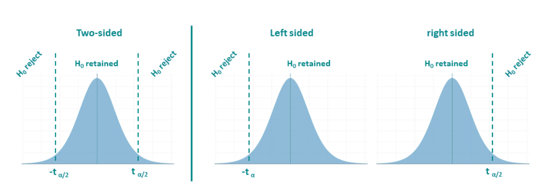
A two-tailed test is the statistical test used for an undirectional hypothesis. Here, extreme values in either direction count as evidence against the null hypothesis, so the rejection regions are split across both tails of the distribution.
In contrast, a one-tailed test is the statistical test that follows from a directional hypothesis. Because the direction is specified in advance, the rejection region lies entirely in one tail of the sampling distribution.
So the mapping is:
An undirectional hypothesis → two-tailed test
A directional hypothesis → one-tailed test
One final but important clarification is that directionality is decided at the hypothesis-formulation stage, not after looking at the data. Choosing a one-tailed test because the observed effect “goes in the expected direction” is statistically invalid.
In short, the terms describe the same distinction, but at different levels:
hypotheses are conceptual, while tails are statistical.
| Non-directional (two-sided) difference hypothesis | Directional (one-sided) difference hypothesis |
|---|---|
|
|
| “There is a difference in salary between men and women.” | “Men earn more than women.” |
| Non-directional correlation hypothesis | Directional correlation hypothesis |
|---|---|
| “There is a correlation between height and weight.” | “The taller a person is, the heavier they are.” A relationship is tested, and the direction (positive) is specified. |
Difference vs. correlation tells you what kind of relationship you are testing;
directional vs. undirectional tells you how specific your prediction is.
Most statistical tests are two-sided by default. Choosing a one-sided test must be done before analysing the data and should be justified by the research context, where only one direction is meaningful.
Every hypothesis test begins with two competing statements about a population parameter.
Null hypothesis (H₀)
The null hypothesis (H₀) represents the default position. It assumes no effect, no difference between groups, or no relationship between variables. Any differences observed in the sample are assumed to be the result of sampling variation alone.
Assumes no effect, no difference, or no relationship in the population.
Any observed difference in the sample is attributed to random sampling variation.
The alternative hypothesis (H₁ or Hₐ) represents what we would conclude if the data provide sufficient evidence against the null hypothesis. It assumes that there is an effect, a difference, or a relationship in the population.
Hypothesis testing does not prove hypotheses true or false.
It helps us decide whether the data provide enough evidence to reject H₀.
Hypothesis testing works by assuming that the null hypothesis is true, and then asking:
How likely is it to observe a result this extreme if H₀ were true?
To answer this, we calculate a test statistic (such as a t value). Test statistics follow known probability distributions under H₀, which allows us to assess how unusual the observed result is.
A hypothesis test produces a test statistic (such as t), which follows a known distribution under H₀.
The p-value is:
The probability of obtaining a result as extreme as, or more extreme than, the observed result, assuming the null hypothesis is true.
A small p-value means the observed result would be unlikely under H₀.
A large p-value means the observed result is plausible under H₀.
To make a decision, we compare the p-value to a significance level (α).
To make decisions consistently, we choose a significance level, denoted by α.
A common choice is α = 0.05. This means that:
if the null hypothesis is actually true,
we are willing to accept a 5% chance of rejecting it by mistake.
****
If p < α, we reject the null hypothesis.
If p ≥ α, we do not reject the null hypothesis.
Rejecting H₀ means the data would be unlikely if H₀ were true.
It does not mean the alternative hypothesis has been proven true.
Importantly, the p-value does not tell us:
the probability that H₀ is true,
the size of an effect,
or whether a result is important in practice.
Hypothesis tests give a decision (reject or do not reject the null hypothesis), but they do not show which values are plausible in the population. For this reason, hypothesis tests should always be accompanied by degrees of freedom and confidence intervals used in the test.
Together, these give a fuller picture of what the data tell us.
Degrees of freedom (df) tell us how many values in our data are genuinely free to vary.
Imagine you have a small set of numbers and you are told what their mean is. Once the mean is fixed, the numbers cannot vary completely freely anymore. Some choices you make automatically restrict the remaining ones.
For example, suppose we have four values and we know their mean is 10. That means the four numbers must add up to 40. You are free to choose the first three values however you like, but once you have chosen them, the fourth value is no longer a choice — it is forced to be whatever number makes the total equal 40. In this situation, only three values are free to vary. The fourth is fixed by the constraint. So we say there are three degrees of freedom, not four.
This is exactly what happens when we calculate variability from a sample. To compute the standard deviation, we first calculate the sample mean. By doing that, we use up one piece of information. The deviations from the mean must sum to zero, so not all deviations are independent. If there are observations, only of them are free to vary once the mean has been fixed.
That is why, when we estimate the population standard deviation from a sample, we divide by rather than . Dividing by would treat all values as fully independent, which they are not once the mean has been estimated. Using corrects for this and gives a more accurate estimate of variability
In short, degrees of freedom count how many independent pieces of information are left after we have estimated something from the data. For variability calculations based on a sample mean, one degree of freedom is lost, leaving .
Suppose we collect a small sample of exam scores:
scores <- c(8, 9, 11, 12)
scores[1] 8 9 11 12First, we calculate the sample size and the sample mean.
n <- length(scores)
mean_score <- mean(scores)

n
[1] 4mean_score[1] 10There are 4 observations, and their mean is 10.
Once the mean is fixed at 10, the four values cannot vary freely anymore. If we change three of the values, the fourth one is forced to take a specific value so that the mean stays the same.
We can see this by calculating the deviations from the mean.
deviations <- scores - mean_score
deviations
[1] -2 -1 1 2Now check what happens when we add the deviations together.
sum(deviations)[1] 0The sum of the deviations is zero. This must always be true once the mean has been calculated. Because of this constraint, not all deviations are independent.
Even though we have 4 observations, only 3 of them are free to vary once the mean is fixed. This is why the degrees of freedom are:
df <- n - 1
df
[1] 3So the degrees of freedom are 3, not 4.
A deviation tells us how far each value is from the mean.
We calculate a deviation by subtracting the mean from each observation:
\[\text{deviation} = x_i - \bar{x}\]
In our example, the mean score is 10.
The deviations are:
These deviations tell us how the data are spread around the mean.
The mean is defined as the balance point of the data.
For every value below the mean, there must be values above the mean to balance it out. As a result:
This is why, once the mean has been calculated, not all deviations are independent. If you know all but one deviation, the final one is already fixed so that the total remains zero.
This constraint is exactly why we lose one degree of freedom when we estimate variability using the sample mean.
A confidence interval (CI) provides a range of values for a population parameter that are compatible with the observed data, given the statistical model.
In the context of an unpaired t-test, the confidence interval is usually reported for the difference in population means.
A 95% confidence interval should be interpreted as follows:
If we were to repeatedly take random samples from the population and construct a confidence interval each time, about 95% of those intervals would contain the true population parameter.
Once a specific confidence interval has been calculated, the true population value is either inside the interval or not. The 95% refers to the long-run reliability of the method, not the probability for a single interval.
To calculate a confidence interval (CI), we need a statistical model for the sampling distribution of the parameter of interest (for example, the population mean).
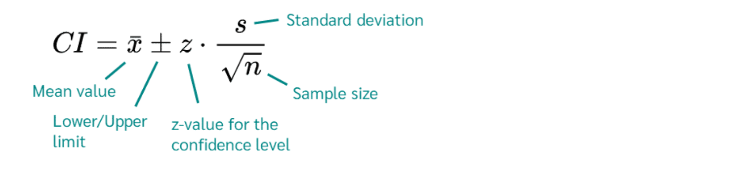
If we assume that the outcome variable is approximately normally distributed in the population, the confidence interval for the mean can be written as:
where:
The \(\pm\) symbol indicates that the confidence interval has a lower limit and an upper limit, centred around the sample mean.
In other words, the confidence interval is constructed by taking the sample mean and extending equally in both directions to reflect sampling uncertainty.
The components of a confidence interval come from two different sources:
the sample data and the statistical model.
The following quantities are calculated directly from the observed sample:
\(\bar{x}\) (sample mean)
Calculated by averaging the observed values in the sample.
\(s\) (sample standard deviation)
Calculated from the spread of the observed data around the sample mean.
\(n\) (sample size)
The number of observations in the sample.
These values summarise what we observed in the sample.
\(z\) (critical value)
This value comes from the normal distribution and depends on the chosen confidence level.
For example:
These values are obtained from probability tables or statistical software, not from the data itself.
The confidence interval combines:
This margin of error depends on:
Sample statistics tell us what we observed.
Distributional theory tells us how uncertain that estimate is.
Together, they allow us to construct a confidence interval that reflects both the data and the uncertainty inherent in sampling.
Confidence intervals help us to:
see which population differences are plausible,
assess the size and direction of an effect,
interpret statistical significance more meaningfully than using a p-value alone.
For example:
A confidence interval that does not include 0 is consistent with a statistically significant difference.
A narrow interval indicates a more precise estimate of the population difference.
In the confidence interval formula, you will sometimes see a \(z\) value and sometimes a \(t\) value. Both play the same role: they determine how wide the confidence interval is. The difference lies in the assumptions we make.
A table is based on the standard normal distribution.
We use a value when the population standard deviation is known. In this case, all uncertainty comes from sampling, and the normal distribution describes that uncertainty exactly.
This leads to the confidence interval formula:
\[CI = \bar{x} \pm z \times \frac{s}{\sqrt{n}}\]
For example, for a 95% confidence interval, the critical value is:
\[z = 1.96\]
This value comes from the z table and captures the middle 95% of the normal distribution.
In practice, this situation is rare, because we almost never know the population standard deviation.
A table works in the same way as a table, but it is used for the distribution.
The key difference is that the distribution:
accounts for the fact that the population standard deviation is unknown, and
depends on the degrees of freedom, which reflect the sample size.
This leads to the confidence interval formula:
\[CI = \bar{x} \pm t \times \frac{s}{\sqrt{n}}\]
Here, the value depends on:
the chosen confidence level, and
the degrees of freedom.
A t table therefore has:
rows for degrees of freedom, and
columns for confidence levels (or tail probabilities)
When you look up \(df\) = 3 and 95% confidence, you find the value 3.18.
When the population standard deviation is unknown, we replace \(z\) with \(t\) in the confidence interval formula.
R does not store these printed tables. Instead, it calculates the same values directly using mathematical formulas.
So:
a z table in a book ↔︎ qnorm() in R
a t table in a book ↔︎ qt() in R
For example:
qnorm(0.975)[1] 1.959964returns the same value you would find in a z table for a 95% CI.
qt(0.975, df = 3)[1] 3.182446returns the same value (about 3.18) you would find in a t table for 3 degrees of freedom.
Suppose we collect a sample of exam scores:
scores <- c(8, 9, 11, 12)
mean(scores)
[1] 10sd(scores)[1] 1.825742length(scores)[1] 4From the data we obtain:
The degrees of freedom are:
\[df = n - 1 = 3\]
For a 95% confidence interval with 3 degrees of freedom, the critical t value is about \(t = 3.18\).
The confidence interval is therefore:
\[10 \pm 3.18 \times \frac{1.83}{\sqrt{4}}\]
\[10 \pm 2.91\]
\[[7.09,\ 12.91]\]
This means that, based on the sample data, plausible values for the population mean lie between 7.09 and 12.91.
When reporting an unpaired t-test, you should include all of the following:
the test statistic (t),
the degrees of freedom (df),
the p-value,
the 95% confidence interval for the mean difference.
These elements work together:
the p-value addresses whether the observed result is unlikely under the null hypothesis,
the confidence interval shows which population values are compatible with the data,
the degrees of freedom indicate how much information the test is based on.
Group A (n = 108, M = 72.5, SD = 6.4) and Group B (n = 92, M = 55.8, SD = 7.1) were compared using an independent-samples t-test.
The difference in means was statistically significant, t(198) = 20.90, p < 0.001.
The 95% confidence interval for the mean difference was [15.1, 18.3].
This suggests that, in the population, the mean outcome differs between the two groups.
Hypothesis testing answers whether a difference is unlikely to be due to chance.
Confidence intervals answer which population values are plausible.
Good statistical reporting always includes both, along with the degrees of freedom that underpin the test.
One of the main sources of confusion in hypothesis testing is language. Many mistakes students describe as “careless” are actually caused by mixing up key terms or using incorrect notation.
Before working with hypothesis tests, it is essential to understand the following concepts clearly.
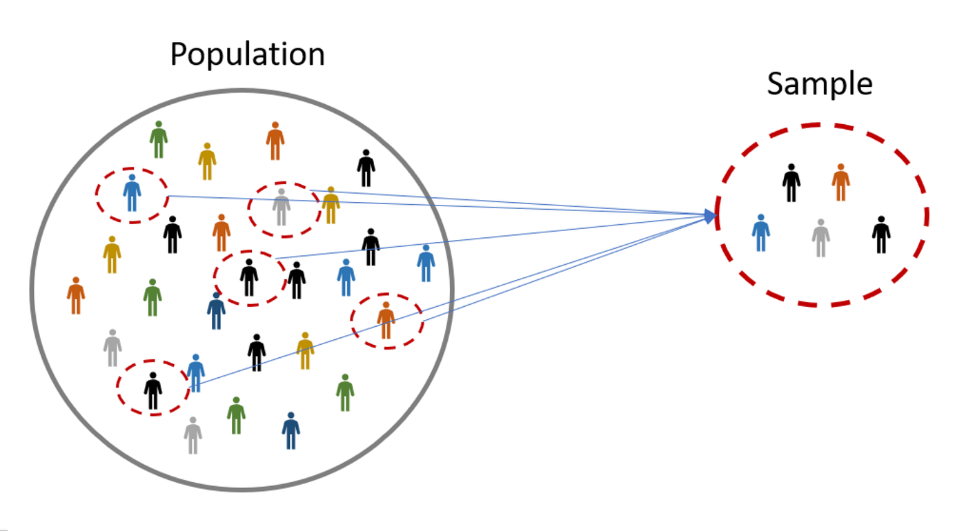
In statistics, we are usually interested in making statements about a population, but we collect data from a sample.
Population
The entire group of individuals, objects, or data values we want to make a statement about.
The population must always be clearly defined.
Sample
A subset of the population from which data are actually collected.
Samples are used because it is often impractical or impossible to measure every member of the population.
In hypothesis testing, it is crucial to keep track of what belongs to the population and what belongs to the sample, because we use different notation for each.
The same words (mean, proportion, standard deviation) are used for both populations and samples, but they do not mean the same thing.
A parameter describes a population
A statistic describes a sample.
Hypotheses are always written about population parameters, even though we calculate sample statistics from the data.
Population quantities are usually unknown.
| Symbol | Meaning |
|---|---|
| \(\mu\) | population mean |
| \(p\) | population proportion |
| \(\sigma\) | population standard deviation |
| \(N\) | population size |
Sample quantities are calculated directly from the data and vary from sample to sample.
| Symbol | Meaning |
|---|---|
| \(\bar{x}\) | sample mean |
| \(\hat{p}\) | sample proportion |
| \(s\) | sample standard deviation |
| \(n\) | sample size |
A very common error is writing hypotheses using sample notation.
Hypotheses must always be written in terms of population parameters.
You do not need to memorise formulas at this stage, but you must understand what each quantity describes.
The average value.
The fraction of individuals with a particular characteristic.
A measure of how spread out the data are.
The context of the problem tells you whether you are dealing with a population or a sample.
You will see the symbols below throughout the course.
It is important to know how to say them aloud and how to write them correctly in R Markdown.
\(\bar{x}\)
Read as: x-bar
Meaning: sample mean
Write in R Markdown as: $\bar{x}$
\(\mu\)
Read as: mu (pronounced myoo)
Meaning: population mean
Write in R Markdown as: $\mu$
\(\hat{p}\)
Read as: p-hat
Meaning: sample proportion
Write in R Markdown as: $\hat{p}$
\(p\)
Read as: p
Meaning: population proportion
Write in R Markdown as: $p$
\(s\)
Read as: s
Meaning: sample standard deviation
Write in R Markdown as: $s$
\(\sigma\)
Read as: sigma
Meaning: population standard deviation
Write in R Markdown as: $\sigma$
The context of the problem tells you whether you are dealing with a population or a sample.