Week 12 – Chi-square Tests

1. When do we use a Chi-square test?

A Chi-square test of independence is used when:

• you have two categorical variables

• you want to know whether they are associated

Key idea

Chi-square tests evaluate whether the pattern of counts in a contingency table is different from what we would expect by chance if the variables were unrelated.

2. Example research question

Remember the research question

Is degree programme related to year of study?

Here we have:

• Degree (categorical, many levels)

• Year (categorical, 3 levels)

Association (relationship) vs causation

In this course we often talk about relationships or associations between variables.
It is important to understand how this differs from causation.

Association (relationship)

Two variables are associated if they tend to vary together.

• When one variable changes, the other tends to change as well
• This can be a positive association, a negative association, or no association
• Association does not imply that one variable causes the other

The Chi-square test of independence tests association only.

Causation

A variable causes another variable if changing the first one directly produces a change in the second.

To claim causation, we usually need: - controlled experiments - random assignment - evidence ruling out alternative explanations

Most observational data do not allow causal conclusions.

Key similarity

• Both association and causation involve relationships between variables

Key difference

Association	Causation
Variables move together	One variable produces change in another
Can be observed in data	Requires strong design and evidence
Tested by Chi-square	Not tested by Chi-square

Example

Suppose we find an association between year of study and average stress level.

• We can say:
  > “Year of study is associated with stress levels.”

• We cannot say:
  > “Being in a higher year causes more stress.”

Why not?

• Students in higher years may have harder courses
  
• They may work more hours
  
• They may differ in age or responsibilities

These factors could explain the association.

Key takeaway

Statistical tests in this course tell us about association, not causation.
We describe results carefully and avoid causal language unless the study design justifies it.

3. Step 1: Create a contingency table (observed frequencies)

We start by counting how many students fall into each Degree × Year combination.

observed_long <- students |>
count(Degree, Year, name = "n")

observed_long

# A tibble: 36 × 3
   Degree       Year      n
   <chr>        <fct> <int>
 1 Anthropology 1         8
 2 Anthropology 2        11
 3 Anthropology 3         3
 4 Architecture 1         1
 5 Architecture 2         3
 6 Architecture 3         3
 7 Business     1         7
 8 Business     2         5
 9 Business     3         3
10 Design       1         2
# ℹ 26 more rows

This is a contingency table in long format. For the Chi-square test, we usually want the classic matrix format:

observed_matrix <- table(students$Degree, students$Year)
observed_matrix

              
                1  2  3
  Anthropology  8 11  3
  Architecture  1  3  3
  Business      7  5  3
  Design        2  9  5
  Education     3  8  6
  English       3  7  2
  History       8  6  6
  Linguistics   6 16  7
  Philosophy    7  6  2
  Politics      5  5  4
  Psychology   11  7  6
  Sociology     2  6  1

Why do we use table() here?

table() creates a contingency table in matrix format (rows × columns), where each cell contains an observed count.

This format is useful because:

• it matches the way contingency tables are shown in textbooks
• it is the format expected by many functions (including chisq.test())
• it makes it easy to see the structure of the data:
  rows = one categorical variable (Degree), columns = the other (Year)

In other words, table() gives us the observed frequencies that the Chi-square test compares to the expected frequencies under the null hypothesis.

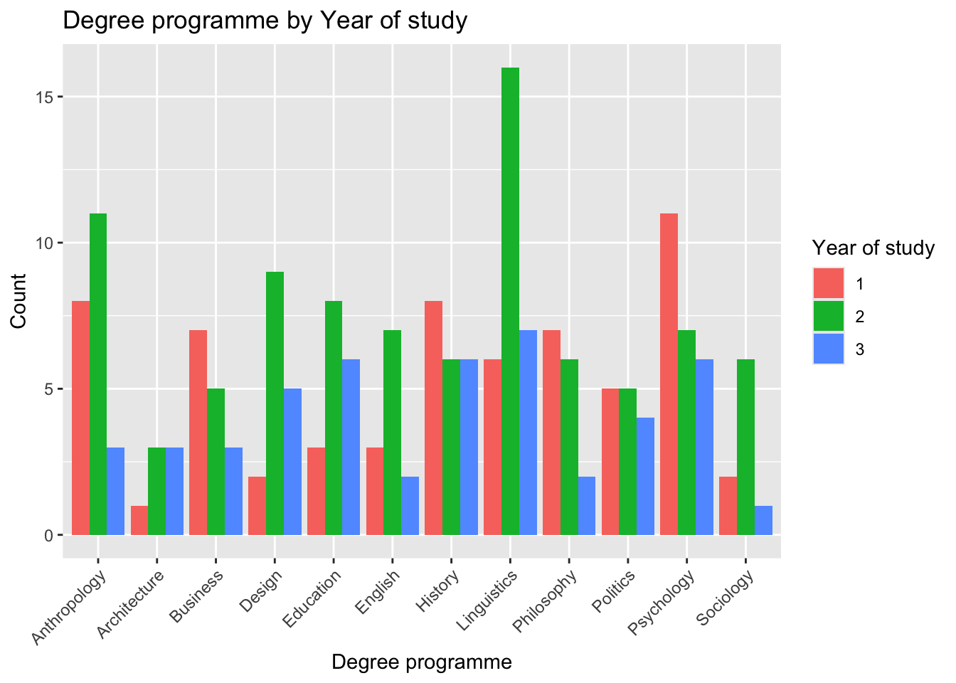
4. Step 2: Visualise the relationship

A grouped bar chart makes it easier to see differences across categories.

ggplot(students, aes(x = Degree, fill = Year)) +
geom_bar(position = "dodge") +
labs(
x = "Degree programme",
y = "Count",
fill = "Year of study",
title = "Degree programme by Year of study"
) +
theme(axis.text.x = element_text(angle = 45, hjust = 1))

Why we plot before testing

A plot helps you see what the data look like, but it does not tell you whether the pattern is likely to exist in the population. That is what hypothesis testing is for.

Check the type of variable before plotting

Before creating a plot or running a test, always check what type of variable you are working with.

• Categorical variables (e.g. Degree, Year) are visualised with bar plots
• Numerical variables (e.g. IQ, Study_hours) are visualised with histograms, boxplots, or density plots

Even if a variable is stored as numbers (e.g. Year = 1, 2, 3), it may still be categorical in meaning and should be treated as a factor.

5. Step 3: State the hypotheses (H₀ and H₁)

Reusable hypothesis template (for reports)

• Null hypothesis (H₀): There is no association between [categorical variable 1] and [categorical variable 2].

• Alternative hypothesis (H₁): There is an association between [categorical variable 1] and [categorical variable 2].

For our example:

• H₀: There is no association between degree programme and year of study.

• H₁: There is an association between degree programme and year of study.

Association, not causation

Chi-square tests do not tell us that one variable causes the other. They only test whether the variables are related in the sample.

Converting numeric variables to categorical (factors)

Sometimes a variable is stored as numbers, but those numbers represent categories, not quantities.

For example, the variable Year may be coded as 1, 2, and 3, but these values do not represent amounts or distances. They represent groups (Year 1, Year 2, Year 3).

In these cases, we should convert the variable to a factor.

Adding meaningful labels (recommended)

We can make the categories easier to interpret by adding labels.

students <- students |>
  mutate(
    Year = factor(
      Year,
      levels = c(1, 2, 3),
      labels = c("Year 1", "Year 2", "Year 3")
    )
  )

students

# A tibble: 200 × 14
   ID    Degree       Year   Gender     Study_hours Sleep_hours Stress_level
   <chr> <chr>        <fct>  <chr>            <dbl>       <dbl> <chr>       
 1 S001  Architecture Year 2 Female             6.8         7.4 Moderate    
 2 S002  Linguistics  Year 1 Male               3.1         5.8 High        
 3 S003  English      Year 2 Female             8.2         7.6 Low         
 4 S004  Philosophy   Year 1 Male               5.5         6.7 Moderate    
 5 S005  Linguistics  Year 2 Non-binary         4           5.9 High        
 6 S006  Linguistics  Year 2 Female             7.4         7.8 Low         
 7 S007  Philosophy   Year 2 Male               2.7         5   High        
 8 S008  Education    Year 3 Female             9           8.2 Low         
 9 S009  Anthropology Year 2 Male               5.9         6.6 Moderate    
10 S010  Sociology    Year 2 Female             6.3         7.1 Moderate    
# ℹ 190 more rows
# ℹ 7 more variables: Satisfaction_Likert_item <chr>,
#   Satisfaction_Likert_value <dbl>, Coffee_per_day <dbl>,
#   Social_media_hr <dbl>, Exercise <chr>, Overall_mark <dbl>, IQ <dbl>

What this code does

• factor() converts a variable into a categorical variable
• levels = c(1, 2, 3) specifies the possible category codes present in the data
• labels = c("Year 1", "Year 2", "Year 3")assigns clear, readable labels to each category

6. Step 4: Run the Chi-square test

We now run a Chi-square test of independence.

chisq_out <- chisq.test(observed_matrix)

Warning in chisq.test(observed_matrix): Chi-squared approximation may be
incorrect

chisq_out

    Pearson's Chi-squared test

data:  observed_matrix
X-squared = 20.752, df = 22, p-value = 0.5361

The output includes:

• X-squared: the Chi-square statistic (χ²)

• df: degrees of freedom

• p-value

What does this code do?

The function chisq.test() performs a Chi-square test of independence using the contingency table stored in observed_matrix.

• Each cell of observed_matrix contains an observed frequency
• The test compares these observed counts to expected frequencies under the null hypothesis of independence
• The output summarises the overall difference using a single χ² statistic

In short, this line asks:
Are the observed counts different from what we would expect if the variables were unrelated?

Why do we save the test as an object?

We assign the result of the test to an object called chisq_out so that we can reuse the information later.

The object chisq_out contains: - the Chi-square statistic (χ²) - the degrees of freedom - the p-value - the expected frequencies for each cell

Saving the test result is essential because we will use chisq_out$expected in the next step to: - inspect expected frequencies - check whether the assumptions of the Chi-square test are met

If we did not save the test as an object, we would have to rerun the test every time we need this information.

Statistical notation used when reporting Chi-square tests

When reporting a Chi-square test, we use standard mathematical symbols.

You will typically see the result written as:

χ²(df) = value, p = value

Where:

• χ² (chi-squared)
  is the Chi-square test statistic (reported in R as X-squared)

• df
  are the degrees of freedom

• p
  is the p-value

For example, if R reports:

• X-squared = 20.75
  
• df = 22
  
• p-value = 0.536

We would write:

χ²(22) = 20.75, p = .54

These symbols are part of standard statistical reporting and should be used in written reports.

7. Step 5: Expected frequencies (assumptions check)

The Chi-square test works best when expected counts are not too small.

We can inspect the expected frequencies:

chisq_out$expected

              
                   1      2    3
  Anthropology 6.930  9.790 5.28
  Architecture 2.205  3.115 1.68
  Business     4.725  6.675 3.60
  Design       5.040  7.120 3.84
  Education    5.355  7.565 4.08
  English      3.780  5.340 2.88
  History      6.300  8.900 4.80
  Linguistics  9.135 12.905 6.96
  Philosophy   4.725  6.675 3.60
  Politics     4.410  6.230 3.36
  Psychology   7.560 10.680 5.76
  Sociology    2.835  4.005 2.16

What does this code show?

The expression chisq_out$expected extracts the expected frequencies from the Chi-square test we previously ran.

These expected frequencies are: - the counts we would expect in each cell of the contingency table
- if the null hypothesis of independence were true

Internally, the Chi-square test: 1. uses the row totals and column totals of the observed table
2. calculates the expected count for each cell under independence
3. stores these values inside the test object (chisq_out)

By inspecting chisq_out$expected, we can check whether the assumptions of the Chi-square test are met.

Expected frequencies: what counts as ‘good enough’?

Rules of thumb:

• Ideally, all expected counts ≥ 5

• A common flexible guideline:

  • no expected count below 1, and

  • no more than 20% of cells below 5

If these conditions are not met, R may warn that the Chi-square approximation may be inaccurate.

If your output shows several expected counts below 5, that typically happens because one variable has many levels (here: Degree), which spreads the data across many cells.

8. Step 6: Interpret the test output

The p-value answers:

If degree and year were truly independent, how likely is it to see a χ² statistic this large (or larger) just by chance?

Decision rule:

• if p < 0.05, reject H₀ (evidence of association)

• if p ≥ 0.05, fail to reject H₀ (not enough evidence)

How to write the conclusion in words

• Reject H₀: “There is evidence of an association between X and Y.”

• Fail to reject H₀: “There is no statistical evidence of an association between X and Y in this sample.”

Reminder: Significance level (α)

The significance level (α) is chosen before running the test.
It sets the threshold for deciding whether a result is statistically significant.

• If the p-value < α, we reject H₀
• If the p-value ≥ α, we fail to reject H₀

In practice, we usually set:

• α = 0.05 (5%)

Common interpretation guidelines

• α < 0.01 → very strong evidence (very significant result)
• α < 0.05 → statistically significant result
• α ≥ 0.05 → not statistically significant

What does α really mean?

The significance level represents the probability of a Type I error.

A Type I error occurs when we reject the null hypothesis even though it is actually true.

For example:

• If α = 0.05, and we reject H₀,
• we accept a 5% chance of making a mistake by claiming an association that does not exist in the population.

Why not always choose a smaller α?

• Lowering α (e.g. to 0.01) reduces the chance of a false positive
• but it also makes it harder to detect real effects

There is always a trade-off between being too strict and too lenient.
This is why α = 0.05 is a widely accepted balance in many fields.

9. Step 7: Effect size (Cramér’s V)

A p-value tells you about evidence, but not strength.

For Chi-square tests we report Cramér’s V.

cramer_v <- cramerV(observed_matrix)
cramer_v

Cramer V 
  0.2278 

This code calculates Cramér’s V, which is the standard effect size measure for a Chi-square test of independence.

• observed_matrix is the contingency table of observed counts

• cramerV() uses the Chi-square statistic and table dimensions to compute a standardised measure of association

• the result is stored in the object cramer_v so it can be:

  • reported in writing

  • compared across analyses

  • interpreted alongside the p-value

Cramér’s V always ranges from 0 to 1.

Interpretation guidelines (rules of thumb):

• around 0.10 = small association

• around 0.30 = moderate association

• around 0.50 = large association

P-values vs effect sizes

A result can be non-significant and still have a non-zero effect size. The p-value is about evidence, while Cramér’s V is about strength.

Note: p-value and Effect size

P-values vs effect sizes

A p-value answers the question:

Is there evidence of an association in the population?

An effect size answers the question:

How strong is that association?

This means:

• a result can be non-significant but still have a non-zero effect size

• a result can be statistically significant but have a very small effect

The p-value is about evidence.
Cramér’s V is about strength.

This is why we always report both.

Statistical significance vs practical significance

A p-value tells us about statistical significance:

Is there evidence of an association in the population, or could this pattern be due to chance?

An effect size (such as Cramér’s V) tells us about practical significance:

How strong or meaningful is the association in real terms?

These are not the same thing.

Why this matters

• A result can be statistically significant but practically trivial
  
• A result can be not statistically significant but still show a noticeable association in the sample

Examples

Example 1: Statistically significant but not practically important

Suppose we analyse data from 10,000 students and find:

• p < 0.001 (statistically significant)
• Cramér’s V = 0.05 (very small effect)

The association exists, but it is so weak that it may not matter in practice.

Example 2: Practically meaningful but not statistically significant

Suppose we analyse data from 40 students and find:

• p = 0.08 (not statistically significant)
• Cramér’s V = 0.30 (moderate effect)

The sample is small, so we lack strong evidence, but the size of the association is meaningful and may be worth further study.

Key takeaway

• Statistical significance is about evidence
• Practical significance is about impact
• Good statistical reporting considers both

This is why we always report both the p-value and the effect size.

10. Reporting (what to write in a report)

A good write-up includes:

• the test name

• χ² statistic

• degrees of freedom

• p-value

• effect size (Cramér’s V)

• a one-sentence conclusion in plain language

Reusable reporting template

A Chi-square test of independence was conducted to examine the relationship between [X] and [Y]. The test showed [a significant / no statistically significant] association, χ²(df) = value, p = value, Cramér’s V = value.

Example reporting sentence (fill in from your output)

You will replace the placeholders with your actual results from chisq_out and cramer_v:

• χ² = 20.75

• df = 22

• p = 0.536

• Cramér’s V = 0.228

A model sentence (edit based on significance):

A Chi-square test of independence was conducted to examine the relationship between degree programme and year of study, χ²(22) = 20.75, p = 0.536, Cramér’s V = 0.228.

11. Glossary

• Contingency table: a table of counts for combinations of two categorical variables.

• Observed frequency: the count we actually see in the data.

• Expected frequency: the count we would expect if the variables were independent.

• Chi-square test of independence: a hypothesis test for association between two categorical variables.

• Degrees of freedom (df): determined by the table size: (rows − 1)(columns − 1).

• p-value: how surprising the χ² statistic is if the null hypothesis is true.

• Cramér’s V: effect size for Chi-square tests (0 to 1).

• Association: a relationship between variables (not causation).
  

Functions used this week:

• count() to create frequency tables

• table() to create contingency tables

• ggplot() + geom_bar() to plot counts

• chisq.test() to run the Chi-square test

• cramerV() to compute Cramér’s V