| Variable Name | Description |
|---|---|
| Name | Name of the institution |
| State | US state where the institution is located |
| ID | Institution ID number |
| Main | Main campus indicator (1 = main campus, 0 = branch campus) |
| Control | Control of institution (Private, Profit, Public) |
| Region | US region (Midwest, Northeast, Southeast, West, etc.) |
| Locale | Locale type (City, Suburb, Town, Rural) |
| Enrollment | Undergraduate enrolment (number of students) |
| AdmitRate | Admission rate (proportion of applicants admitted) |
| Cost | Average total cost (tuition, room, board, etc.) |
| PartTime | Percent of undergraduates who are part-time students |
| TuitionIn | In-state tuition and fees |
| TuitionOut | Out-of-state tuition and fees |
Numeric data– MSDA IFP
Week 10 – Tutorial 03 Continuous Variables
1. Tasks For formative report
This week’s task is highlighted in bold below. Please only focus on completing that task this week. In the next section, you will also find guided sub-steps you may want to consider to complete this week’s task.
- Read the College dataset into R, inspect it, and write a concise introduction to the data and its structure.
- Display and describe the categorical variables.
3) Display and describe a selection of numeric variables.
- Display and describe at least one relationship between two variables.
- Finish the report write-up, knit to PDF, and submit.
This tutorial is designed to help you complete Task 3.
1.1 Task 3 – sub-tasks
Tip
Tip: Hover over the footnotes for hints showing useful R functions.
This week you will only focus on Task 3: Display and describe a selection of numeric variables.
Below there are some guided sub-steps you may want to consider to complete Task 3, following the same structure required in Assessment Stage 1.
- Reopen last week’s
.qmdfile, as you will continue last week’s work and build on it.1
Read the CollegeScores dataset into R (from the provided CSV file in
datasets/) and give the object a sensible name (for examplecollege).2Use functions such as
glimpse()orstr()to check the structure of the dataset (what variables exist and how is R reading them - characters, factor, numeric, etc.) and identify which variables are numeric and suitable for descriptive analysis.3Describe the following numeric variables
Enrolment,AdminRateandCost.4For each numeric variable, complete the following steps separately, using a new subheading titled with the variable name exactly as it appears in the dataset:
- Identify the variable
- State what the variable measures.
- Identify its level of measurement.
- Briefly justify this classification.
- Explore the distribution
- Begin by exploring the distribution of the variable.
- Create one plot that is appropriate for describing this variable.
- Explain why this plot is suitable.
- Describe the distribution shape
- Describe the observed shape of the distribution (e.g. symmetric, right-skewed).
- Explain what this tells you about the data.
- Choose numerical summaries
- Report appropriate numerical summaries.
- Justify your choice of summaries based on:
- the level of measurement, and
- the observed shape of the distribution.
- Interpretation
- Interpret the plot and numerical summaries together.
- Describe the typical values and the variability of the variable in the dataset.
When choosing your plot:
- use a histogram for continuous numeric variables,
- consider a boxplot if you want to emphasise the median and interquartile range,
Repeat this process for each numeric variable you have selected.
In your written Analysis section:
- do not refer to R code or functions,
- focus on explaining what the plot and summaries reveal about the data,
- ensure your reasoning is clear, logical, and explicit.
You do not need to include R output in the report; you only need the written description.
Keep this paragraph; you will re-use it in your report.
Data
CollegeScores Dataset
You will work with the CollegeScores dataset in this tutorial.
At the link CollegeScores_teaching.csv you will find information about 400 higher-education institutions in the United States.
The dataset includes variables describing each institution’s location, sector (public/private), tuition costs, enrolment, and the demographic composition of their student body.
For this tutorial, analyse the following numeric variables:
Enrollment(undergraduate enrolment)AdmitRate(admission rate)Cost(average total cost)
library(tidyverse)── Attaching core tidyverse packages ──────────────────────── tidyverse 2.0.0 ──
✔ forcats 1.0.1 ✔ readr 2.2.0
✔ ggplot2 4.0.2 ✔ stringr 1.6.0
✔ lubridate 1.9.5 ✔ tidyr 1.3.2
✔ purrr 1.2.1
── Conflicts ────────────────────────────────────────── tidyverse_conflicts() ──
✖ dplyr::filter() masks stats::filter()
✖ dplyr::lag() masks stats::lag()
ℹ Use the conflicted package (<http://conflicted.r-lib.org/>) to force all conflicts to become errorscollege <- read_csv("CollegeScores_teaching.csv")Rows: 400 Columns: 17
── Column specification ────────────────────────────────────────────────────────
Delimiter: ","
chr (5): Name, State, Control, Region, Locale
dbl (12): ID, Main, Enrollment, PartTime, TuitionIn, TuitionOut, White, Blac...
ℹ Use `spec()` to retrieve the full column specification for this data.
ℹ Specify the column types or set `show_col_types = FALSE` to quiet this message.glimpse(college)Rows: 400
Columns: 17
$ ID <dbl> 101189, 101569, 101693, 105534, 106148, 106625, 107220, 107…
$ Name <chr> "Faulkner University", "Lawson State Community College", "U…
$ State <chr> "AL", "AL", "AL", "AZ", "AZ", "AR", "AR", "AR", "AR", "AR",…
$ Main <dbl> 1, 1, 1, 1, 1, 1, 1, 1, 1, 1, 1, 1, 1, 1, 1, 1, 1, 1, 1, 1,…
$ Control <chr> "Private", "Public", "Private", "Profit", "Public", "Public…
$ Region <chr> "Southeast", "Southeast", "Southeast", "West", "West", "Sou…
$ Locale <chr> "City", "City", "Rural", "City", "City", "Rural", "City", "…
$ Enrollment <dbl> 2272, 3034, 1276, 2300, 4682, 1216, 169, 50, 642, 106, 2908…
$ PartTime <dbl> 23.3, 43.1, 9.7, 0.0, 65.1, 27.3, 0.0, 0.0, 42.7, 18.9, 80.…
$ TuitionIn <dbl> 20970, 4440, 22210, 12992, 2280, 3120, 13695, 15825, 3680, …
$ TuitionOut <dbl> 20970, 8010, 22210, 12992, 8976, 5448, 13695, 15825, 6530, …
$ White <dbl> 41.5, 14.9, 61.7, 39.5, 46.2, 93.3, 75.7, 2.0, 70.6, 85.9, …
$ Black <dbl> 49.7, 80.8, 18.6, 6.4, 0.9, 2.6, 7.7, 98.0, 19.5, 2.8, 7.8,…
$ Hispanic <dbl> 2.0, 1.6, 2.1, 39.0, 26.7, 1.9, 11.8, 0.0, 4.5, 8.5, 24.7, …
$ Asian <dbl> 0.4, 0.8, 1.4, 5.2, 0.7, 0.1, 1.8, 0.0, 0.5, 0.9, 10.6, 2.3…
$ Other <dbl> 6.5, 2.0, 16.2, 10.0, 25.6, 2.1, 3.0, 0.0, 5.0, 1.9, 17.3, …
$ AdmitRate <dbl> 0.5101, NA, 0.4702, NA, NA, NA, NA, NA, NA, NA, NA, NA, 0.6…2 Worked Example
Consider the dataset provided in datasets/HollywoodMovies.csv, containing 1295 observations on the following 15 variables:
| Variable Name | Description |
|---|---|
| Movie | Title of the movie |
| LeadStudio | Primary U.S. distributor |
| RottenTomatoes | Critics' rating (Rotten Tomatoes) |
| AudienceScore | Audience rating (Rotten Tomatoes) |
| Genre | Film genre (e.g., Action Adventure, Comedy, Thriller) |
| TheatersOpenWeek | Number of screens on opening weekend |
| OpeningWeekend | Opening weekend gross (in millions) |
| BOAvgOpenWeekend | Average box office income per theatre, opening weekend |
| Budget | Production budget (in millions) |
| DomesticGross | U.S. gross income (in millions) |
| ForeignGross | Foreign gross income (in millions) |
| WorldGross | Worldwide gross income (in millions) |
| Profitability | Worldwide gross as a percentage of budget |
| OpenProfit | Percentage of budget recovered on opening weekend |
| Year | Year of release |
These data were compiled from Box Office Mojo, The Numbers, and Rotten Tomatoes.
We load the tidyverse package as we will use the functions
read_csv() and glimpse() from this package.
Load tidyverse and import the data
library(tidyverse)
library(kableExtra)
read_csv() reads CSV (comma-separated values) files.
The loaded data are stored in an object called movies using the arrow <-.
movies <- read_csv("HollywoodMovies.csv")movies <- movies |>
select(1:15)
glimpse(movies)Rows: 1,295
Columns: 15
$ Movie <chr> "2016: Obama's America", "21 Jump Street", "A Late Qu…
$ LeadStudio <chr> "Rocky Mountain Pictures", "Sony Pictures Releasing",…
$ RottenTomatoes <dbl> 26, 85, 76, 90, 35, 27, 91, 56, 11, 44, 93, 63, 87, 9…
$ AudienceScore <dbl> 73, 82, 71, 82, 51, 72, 62, 47, 47, 63, 82, 51, 63, 9…
$ Genre <chr> "Documentary", "Comedy", "Drama", "Drama", "Horror", …
$ TheatersOpenWeek <dbl> 1, 3121, 9, 7, 3108, 3039, 132, 245, 2539, 3192, 3, 1…
$ OpeningWeekend <dbl> 0.03, 36.30, 0.08, 0.04, 16.31, 24.48, 1.14, 0.70, 11…
$ BOAvgOpenWeekend <dbl> 30000, 11631, 8889, 5714, 5248, 8055, 8636, 2857, 449…
$ Budget <dbl> 3.0, 42.0, NA, NA, 68.0, 12.0, NA, 7.5, 35.0, 50.0, 1…
$ DomesticGross <dbl> 33.35, 138.45, 1.56, 1.55, 37.52, 70.01, 1.99, 3.01, …
$ WorldGross <dbl> 33.35, 202.81, 6.30, 7.60, 137.49, 82.50, 3.59, 8.54,…
$ ForeignGross <dbl> 0.00, 64.36, 4.74, 6.05, 99.97, 12.49, 1.60, 5.53, 9.…
$ Profitability <dbl> 1334.00, 482.88, NA, NA, 202.19, 687.50, NA, 113.87, …
$ OpenProfit <dbl> 1.20, 86.43, NA, NA, 23.99, 204.00, NA, 9.33, 32.57, …
$ Year <dbl> 2012, 2012, 2012, 2012, 2012, 2012, 2012, 2012, 2012,…We will focus on the following numeric variables:
Budget(production budget, in millions)AudienceScore(audience rating)
2.1 Budget
a. Identification of the variable
- initial exploration of the variable
movies |>
  summarise(
    n_total   = n(),
    n_missing = sum(is.na(Budget)),
    n_valid   = sum(!is.na(Budget))
  )
# A tibble: 1 × 3
n_total n_missing n_valid
<int> <int> <int>
1 1295 239 1056
Understanding
!is.na(Budget)
In R, missing values are stored as NA.
is.na(Budget)checks each value ofBudgetand returns:TRUEif the value is missing
FALSEif the value is present
The symbol ! means “not”.
So:
!is.na(Budget)returnsTRUEfor values that are not missing, andFALSEfor missing values.
When we write:
{sum(!is.na(Budget))}
R counts how many valid (non-missing) budget values there are, because
TRUEis treated as 1FALSEis treated as 0
Adding them up gives the number of observations that can actually be used in plots and numerical summaries.
Being explicit about valid and missing values is good practice, as it makes clear how much data each analysis is based on.
Budget measures the production budget of a movie, expressed in millions of US dollars.
It is a continuous numeric variable, as it represents measured quantities on a continuous scale where differences between values are meaningful.
The dataset contains 1295 movies in total. Of these, 239 movies have missing budget values, leaving 1056 movies with a recorded production budget. All numerical summaries and plots for Budget are therefore based on these 1056 valid observations.
Being explicit about the total number of observations, the number of missing values, and the number of valid cases is an important part of describing a variable. This information helps the reader assess the reliability, coverage, and limitations of the descriptive statistics and visualisations that follow.
b. Exploration of the distribution
To explore the distribution of Budget, we begin with a histogram, which is appropriate for continuous numeric variables and allows us to assess the overall shape of the distribution.
ggplot(movies, aes(x = Budget)) +
  geom_histogram(bins = 25, colour = "white") +
  labs(
    x = "Production budget (millions of USD)",
    y = "Count"
  )
Warning: Removed 239 rows containing non-finite outside the scale range
(`stat_bin()`).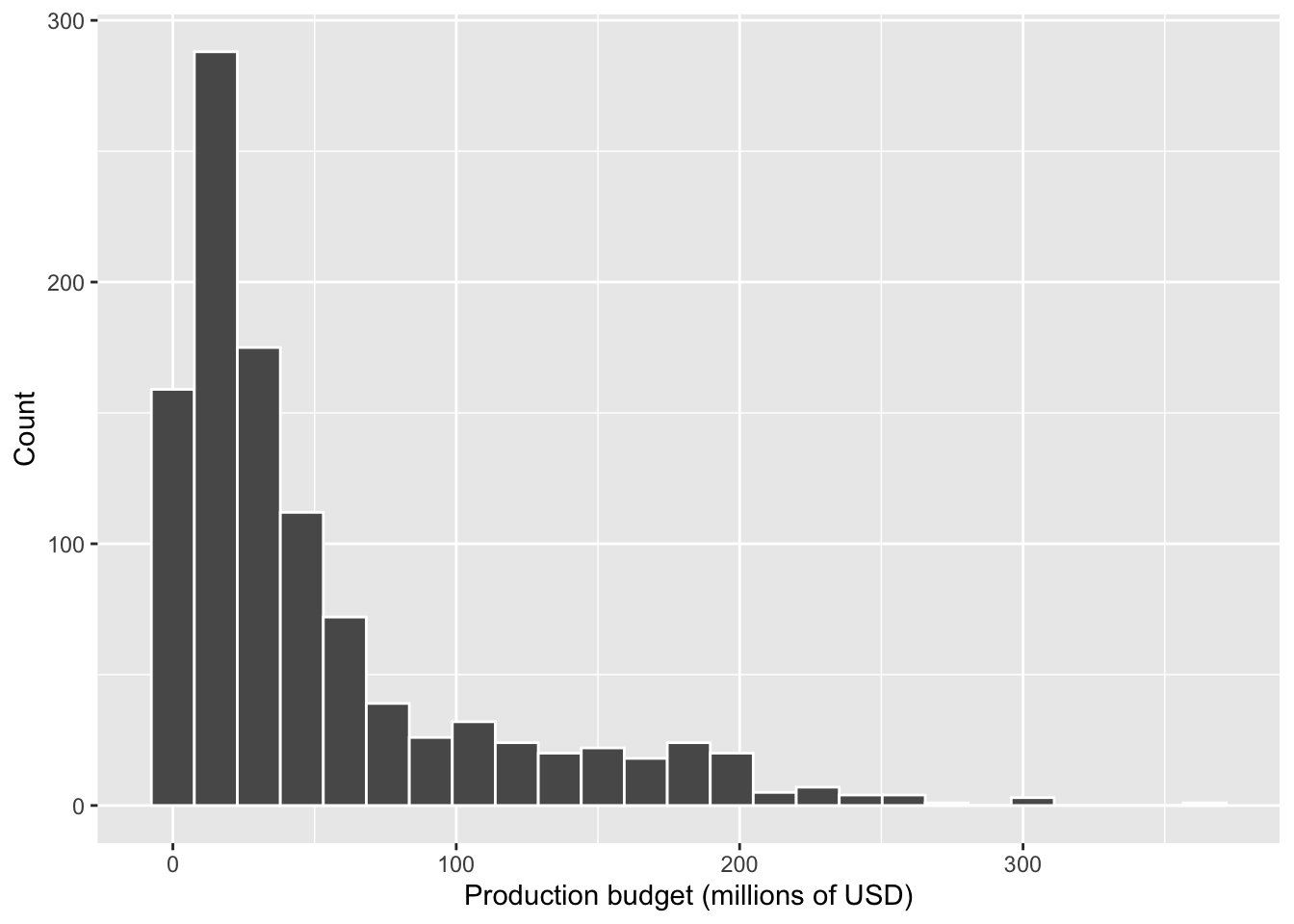
A histogram is suitable here because it shows how movie budgets are distributed across value ranges, making it easy to see patterns such as clustering, skewness, and extreme values.
Why do we see a warning about removed rows?
Some movies in the dataset do not have recorded values for Budget (i.e. the value is missing, or NA).
When we create a histogram, ggplot() automatically excludes missing values, because they cannot be placed into bins.
As a result, ggplot prints a warning such as:
“Removed X rows containing non-finite values”
This is informative, not an error. It simply tells us that: - some observations have missing values, and
- the plot is based only on the available data.
We do not need to remove rows manually at this stage.
Optional: Adding a density curve
Sometimes it is helpful to overlay a density curve on top of a histogram.
A density curve provides a smoothed representation of the
distribution’s shape, which can make features such as skewness and
peakedness easier to see.
To combine a histogram and a density curve, we rescale the histogram so
that it is plotted on the density scale rather than raw counts.
ggplot(movies, aes(x = Budget)) +
  geom_histogram(aes(y = after_stat(density)),
                 bins = 25, colour = "white") +
  geom_density(linewidth = 1) +
  labs(
    x = "Production budget (millions of USD)",
    y = "Density"
  )
Warning: Removed 239 rows containing non-finite outside the scale range
(`stat_bin()`).Warning: Removed 239 rows containing non-finite outside the scale range
(`stat_density()`).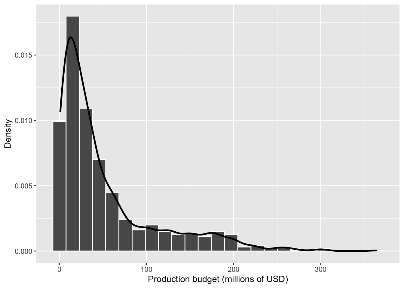
The density curve can make skewness easier to see, especially when the distribution has a long tail.
Skewness and kurtosis in this course
In the lecture, you learned that the shape of a distribution can be described using:
- Skewness (asymmetry: left- or right-skewed), and
- Kurtosis (how peaked the distribution is and how heavy the tails are).
In this tutorial and in Assessment Stage 1, you are not required to calculate or formally report kurtosis.
Instead, you should:
- comment on skewness when it is clearly visible, and
- focus on choosing appropriate plots and numerical summaries.
Kurtosis is introduced to help you understand distributional shape, not as a quantity you need to compute or interpret in your report.
c. Description of the distribution shape
The distribution of production budgets is right-skewed, with most movies concentrated at lower budget values and a long tail extending towards very high budgets.
Although the majority of observations appear on the left-hand side of the plot, the presence of a few extremely large budgets stretches the distribution to the right.
d. Choice of numerical summaries
The purpose of numerical summaries is to describe both the typical value of production budgets and the variability in those budgets across movies.
Because the histogram shows that the distribution of Budget is right-skewed, with a small number of very large values, different summaries serve different roles:
- The mean summarises the overall average budget, and the standard deviation describes how much budgets vary around that average. However, both are influenced by extreme high-budget films.
- The median summarises the central tendency of the distribution in a way that is robust to extreme values, making it a better indicator of a “typical” movie budget in this case.
Reporting both the mean (with standard deviation) and the median allows us to: - capture the overall scale of movie budgets, and - provide a more representative measure of central tendency given the skewed distribution.
Together, these summaries give a more complete and informative description of the data than any single statistic alone.
movies |>
  summarise(
    n = sum(!is.na(Budget)),
    Mean = mean(Budget, na.rm = TRUE),
    SD = sd(Budget, na.rm = TRUE),
    Median = median(Budget, na.rm = TRUE),
    Min = min(Budget, na.rm = TRUE),
    Max = max(Budget, na.rm = TRUE)
  ) |>
  pivot_longer(
    cols = everything(),
    names_to = "Statistic",
    values_to = "Value"
  ) |>
  kbl(
    booktabs = TRUE,
    digits = 2,
    col.names = c("Statistic", "Value")
)| Statistic | Value |
|---|---|
| n | 1056.00 |
| Mean | 51.38 |
| SD | 57.93 |
| Median | 30.00 |
| Min | 0.90 |
| Max | 365.00 |
Understanding how missing values are handled in the code
In the summary table above, two pieces of code are used to deal with missing values (NAs). These do different but complementary things.
1. !is.na(Budget)
is.na(Budget)checks each value ofBudgetand returnsTRUEif the value is missing andFALSEotherwise.- The
!symbol means “not”, so!is.na(Budget)returnsTRUEfor values that are not missing. - When we write
sum(!is.na(Budget)),
R counts how many non-missing budget values there are, because:TRUEis treated as 1FALSEis treated as 0
This gives us the sample size (n) actually used to compute the summaries.
2. na.rm = TRUE
- By default, summary functions such as
mean(),sd(), andmedian()returnNAif any missing values are present. - Setting
na.rm = TRUEtells R to remove missing values before performing the calculation. - This ensures that each statistic is calculated using only the available data.
Importantly, this does not delete rows from the dataset.
It only affects how the summary statistics are computed.
e. Interpretation
Taken together, the histogram and the numerical summaries show that movie production budgets are typically relatively modest, with a small number of very high-budget films. The median budget is $30 million, indicating that half of the movies in the dataset were produced with budgets below this value. This median is substantially lower than the mean budget of $51.38 million, which reflects the right-skewed shape observed in the histogram. The mean is pulled upward by a small number of extremely expensive productions. The variability in budgets is large, as shown by the standard deviation of $57.93 million and the wide range of values. Budgets range from a minimum of $0.9 million to a maximum of $365 million, confirming the presence of extreme high-budget outliers. Overall, most movies cluster at the lower end of the budget scale, while a few blockbuster films account for the long right tail of the distribution. This explains why the median provides a more representative measure of a “typical” movie budget than the mean.
2.2 AudienceScore
a. Identification of the variable
Initial exploration of the variable
movies |>
  summarise(
    n_total   = n(),
    n_missing = sum(is.na(AudienceScore)),
    n_valid   = sum(!is.na(AudienceScore))
  )
# A tibble: 1 × 3
n_total n_missing n_valid
<int> <int> <int>
1 1295 0 1295AudienceScore measures the audience rating of a movie on Rotten Tomatoes, expressed as a percentage score.
It is a continuous numeric variable, as it represents measured values on a numeric scale where differences between values are meaningful.
The dataset contains 1295 movies in total. Some observations have missing audience scores, meaning that only the non-missing values are used in the analyses that follow.
Being explicit about the number of valid observations helps clarify the basis on which summaries and plots are computed.
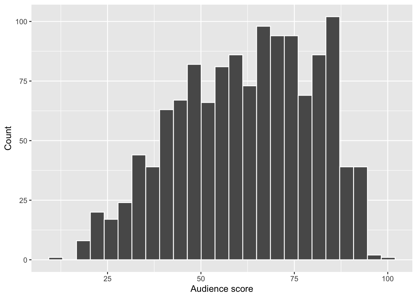
b. Exploration of the distribution
To explore the distribution of AudienceScore, we use a histogram, which is appropriate for continuous numeric variables and allows us to assess the overall shape of the distribution.
ggplot(movies, aes(x = AudienceScore)) +
  geom_histogram(bins = 25, colour = "white") +
  labs(
    x = "Audience score",
    y = "Count"
  )
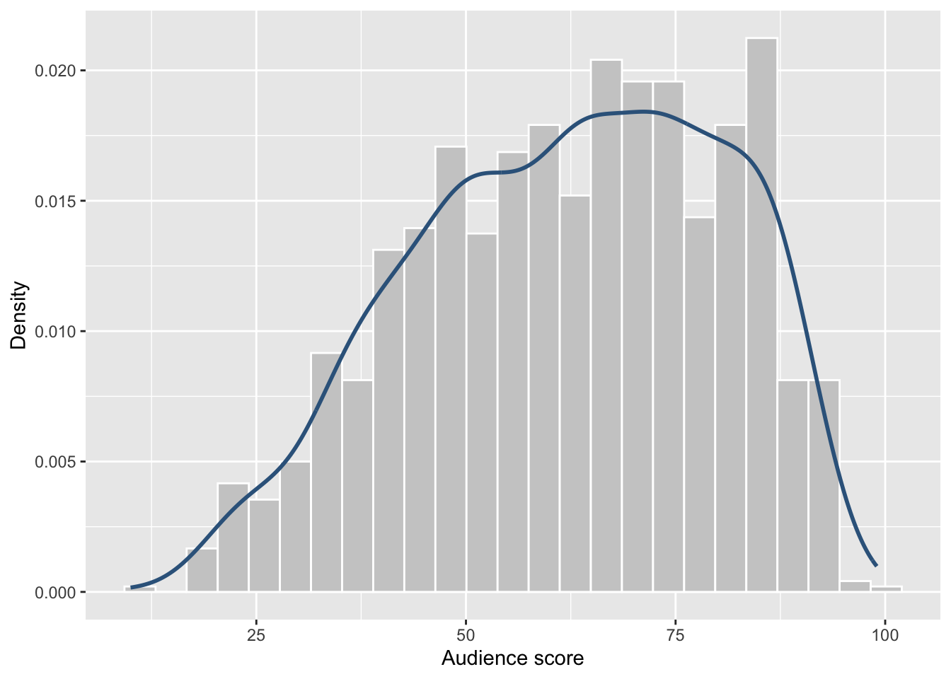
We also overlay a density curve, which provides a smooth representation of the distribution’s shape and makes skewness easier to see.
ggplot(movies, aes(x = AudienceScore)) +
  geom_histogram(
    aes(y = after_stat(density)),
    bins = 25,
    colour = "white",
    fill = "grey80"
  ) +
  geom_density(
    colour = "steelblue4",
    linewidth = 1
  ) +
  labs(
    x = "Audience score",
    y = "Density"
  )
A histogram is suitable here because it shows how audience ratings are distributed across score ranges.
The density curve complements the histogram by smoothing out random variation caused by binning, making the overall shape of the distribution easier to interpret.
Note
Why do we rescale the histogram to density?
By default, histograms display counts on the y-axis, while density curves are scaled so that the total area under the curve equals 1.
Setting
aes(y = after_stat(density))
rescales the histogram to the same density scale as the curve. This allows both layers to be plotted together and interpreted consistently.
What does “symmetric” mean?
A distribution is symmetric if:
- the left and right sides are mirror images of each other,
- the centre of the distribution lies in the middle of the range, and
- the tails extend equally in both directions.
In a symmetric distribution: - the mean, median, and mode are approximately equal, and - the overall shape looks balanced around the centre.
A common example of a symmetric distribution is the normal (bell-shaped) distribution.
c. Description of the distribution shape
The distribution of audience scores is slightly negatively skewed (left-skewed).
Most movies receive moderate to high audience ratings, with scores clustering between approximately 50 and 85.
There are relatively few movies with very low audience scores, which results in a longer tail on the lower end of the distribution. Scores close to the upper bound of 100 are also less common, reflecting the bounded nature of the rating scale.
Overall, this shape indicates that audience ratings tend to be generally favourable, with extreme negative ratings occurring relatively infrequently.
Why is AudienceScore not symmetric?
Although the distribution may appear roughly bell-shaped at first glance, it is not truly symmetric.
There are three key reasons:
1. The centre is not balanced
Most movies receive audience scores towards the higher end of the scale (approximately 60–85), rather than being centred evenly around the midpoint.
If the distribution were symmetric, we would expect: - similar frequencies at scores such as 40 and 80, and - similar behaviour on both sides of the centre.
This is not observed.
2. The tails are unequal
- The left tail (lower scores) extends further and more gradually.
- The right tail drops off more sharply.
Unequal tail lengths are a clear visual indicator of skewness.
3. The scale is bounded
Audience scores are measured on a 0–100 scale, meaning values cannot exceed 100.
This compresses high scores and makes perfect symmetry unlikely, even if the distribution looks smooth.
How can you tell if a distribution is symmetric?
Students can use this simple checklist:
Look at the centre
Is the bulk of the data centred in the middle of the range?Compare the tails
Do both tails extend roughly the same distance?Compare mean and median (if available)
- mean ≈ median → roughly symmetric
- mean < median → left-skewed
- mean > median → right-skewed
- mean ≈ median → roughly symmetric
For AudienceScore, the longer left tail and the imbalance around the centre indicate slight negative skew, rather than symmetry.
d. Choice of numerical summaries
The purpose of numerical summaries is to describe both the typical value of audience ratings and the variability in those ratings across movies.
Because audience scores are measured on a bounded numeric scale (0–100) and the distribution is slightly negatively skewed, no single summary statistic fully captures the distribution.
The mean provides an overall average audience score, and the standard deviation describes how much individual ratings tend to vary around that average. However, the mean is sensitive to skewness and to values near the bounds of the scale.
The median provides a measure of central tendency that is less affected by skewness, making it a more representative indicator of a “typical” audience score in this case.
Reporting both the mean (with standard deviation) and the median allows us to:
summarise the overall level of audience ratings, and
account for the asymmetry of the distribution and the bounded scale.
Together, these numerical summaries give a more complete and informative description of audience ratings than any single statistic alone.
movies |>
  summarise(
    n      = sum(!is.na(AudienceScore)),
    Mean   = mean(AudienceScore, na.rm = TRUE),
    SD     = sd(AudienceScore, na.rm = TRUE),
    Median = median(AudienceScore, na.rm = TRUE),
    Min    = min(AudienceScore, na.rm = TRUE),
    Max    = max(AudienceScore, na.rm = TRUE)
  ) |>
  pivot_longer(
    cols = everything(),
    names_to = "Statistic",
    values_to = "Value"
  ) |>
  kbl(
    booktabs = TRUE,
    digits = 2,
    col.names = c("Statistic", "Value")
)| Statistic | Value |
|---|---|
| n | 1295.00 |
| Mean | 62.18 |
| SD | 18.21 |
| Median | 64.00 |
| Min | 10.00 |
| Max | 99.00 |
What does this part of the code do?
pivot_longer(
  cols = everything(),
  names_to = "Statistic",
  values_to = "Value"
) |>
kbl(
  booktabs = TRUE,
  digits = 2,
  col.names = c("Statistic", "Value")
)
This part of the code is about presentation, not calculation. pivot_longer() By default, summarise() produces a wide table, where each statistic is its own column:
n Mean SD Median Min Maxpivot_longer() reshapes this wide table into a long format, with:
one column for the name of the statistic
one column for the value of that statistic
Specifically:
cols = everything()
→ take all columns produced bysummarise()names_to = "Statistic"
→ store the column names (e.g. Mean, SD, Median) in a new column calledStatisticvalues_to = "Value"
→ store the numerical values in a column calledValue
Statistic   Value
Mean        51.38
SD          57.93
Median      30.00
This format is often easier to read and easier to discuss in text, especially in reports.
kbl()
The kbl() function (from the knitr package) is used to format the table nicely for the report:
booktabs = TRUE
→ improves table spacing and line quality (LaTeX-style tables)digits = 2
→ rounds values to two decimal placescol.names = c("Statistic", "Value")
→ sets clear, reader-friendly column names
Key point
None of this code changes the data or the statistics themselves.
It only changes how the results are displayed in the final report.
e. Interpretation
Taken together, the histogram, density plot, and numerical summaries show that audience ratings are generally moderate to high, with relatively few extremely low scores.
The median audience score is 64, meaning that half of the movies received audience ratings below 64 and half received ratings above this value. The mean score is slightly lower, at 62.18, which is consistent with the slight negative (left) skew observed in the distribution. This indicates that a small number of lower-rated movies pull the mean downward.
The standard deviation of 18.21 shows that audience scores vary moderately around the average, suggesting meaningful differences in how audiences rate different films. Scores range from a minimum of 10 to a maximum of 99, indicating that while extremely poor or near-perfect ratings do occur, they are relatively uncommon.
Overall, most movies receive fairly favourable audience ratings, clustering toward the upper-middle of the scale. Because of the slight skew and the bounded nature of the rating scale, the median provides a slightly more representative measure of a typical audience score than the mean, although reporting both gives a fuller picture of the distribution.
3 Wrap-up: Task 3 (numeric variables) — what you should be able to do
By the end of this tutorial, you should be able to:
Write your Stage 1 descriptive statistics for a numeric variable by
(1) checking missing data,
(2) exploring the distribution with a plot,
(3) describing the shape,
(4) choosing summaries that match the shape, and
(5) interpreting the plot and summaries together.
3.1 Quick reference: commands you used in this tutorial
This table is here so you can quickly find the command you need when you get stuck.
| Goal | Typical command(s) |
|---|---|
| Load packages | library(tidyverse) |
| Read a CSV file | read_csv("CollegeScores_teaching.csv") |
| Check the structure (variable types) | glimpse(college) or str(college) |
| Select variables | select(Enrollment, AdmitRate, Cost) |
| Check missing values and valid n | summarise(n_total = n(), n_missing = sum(is.na(x)), n_valid = sum(!is.na(x))) |
| Histogram (numeric distribution) | ggplot(data, aes(x = x)) + geom_histogram() |
| Boxplot (median + IQR view) | ggplot(data, aes(y = x)) + geom_boxplot() |
| Mean / SD | mean(x, na.rm = TRUE) , sd(x, na.rm = TRUE) |
| Median / IQR | median(x, na.rm = TRUE) , IQR(x, na.rm = TRUE) |
| Min / Max | min(x, na.rm = TRUE) , max(x, na.rm = TRUE) |
| Make a summary table | summarise(...) |
| Make a “long” table for reporting | pivot_longer(cols = everything(), ...) |
| Format a table nicely | kbl(...) |
Footnotes
Hint: Open the same
.qmdfile you used for Task 1 so you keep building a single report.↩︎Hint: Use
read_csv("datasets/CollegeScores_teaching.csv")from the readr package.↩︎Hint: Try
glimpse(college)from dplyr orstr(college).↩︎Hint: Numeric variables include costs, percentages, counts, and scores stored as numbers.↩︎