| Variable Name | Description |
|---|---|
| Name | Name of the institution |
| State | US state where the institution is located |
| ID | Institution ID number |
| Main | Main campus indicator (1 = main campus, 0 = branch campus) |
| Control | Control of institution (Private, Profit, Public) |
| Region | US region (Midwest, Northeast, Southeast, West, etc.) |
| Locale | Locale type (City, Suburb, Town, Rural) |
| Enrollment | Undergraduate enrolment (number of students) |
| AdmitRate | Admission rate (proportion of applicants admitted) |
| Cost | Average total cost (tuition, room, board, etc.) |
| PartTime | Percent of undergraduates who are part-time students |
| TuitionIn | In-state tuition and fees |
| TuitionOut | Out-of-state tuition and fees |
– MSDA IFP
Week 12 – Tutorial 05 Chi-squared Test
1. Tasks for formative report
This week’s task is highlighted in bold below. Please only focus on completing that task this week. In the next section, you will also find guided sub-steps you may want to consider to complete this week’s task.
- Read the College dataset into R, inspect it, and write a concise introduction to the data and its structure.
- Display and describe the categorical variables.
- Display and describe a selection of numeric variables.
4) Test at least one research question using an appropriate hypothesis test.
- Finish the report write-up, knit to PDF, and submit.
This tutorial is designed to help you complete Task 4.
1.1 Task 4 – sub-tasks
Tip
Tip: Hover over the footnotes for hints showing useful R functions.
This week you will focus on Task 4: Test at least one research question using an appropriate hypothesis test.
Below are guided sub-steps you may want to follow, using the structure required in Assessment Stage 2.
Your required structure for each research question
For each research question, you must complete these steps in order:
- State the research question in your own words.
- Write the null hypothesis (\(H_0\)) and the alternative hypothesis (\(H_1\)).
- Identify the variables involved and their roles (grouping variable, outcome variable).
- Consider which statistical test is appropriate, and justify your choice.
- Prepare the data only as required to answer the research question
(minimal subsetting only where necessary).
- Conduct the statistical analysis in R.
- Report the relevant statistical output
(t, df, p-value, and confidence interval).
- Produce one appropriate visualisation and refer to it in the text.
Your writing should be clear and concise.
Interpretation should be brief and factual.
Data
CollegeScores Dataset
You will work with the CollegeScores dataset in this tutorial.
At the link CollegeScores_teaching.csv you will find information about 400 higher-education institutions in the United States.
The dataset includes variables describing each institution’s location, sector (public/private), tuition costs, enrolment, and the demographic composition of their student body.
Research questions for this tutorial
For Task 4, you must answer the following research questions using a Chi-square test of independence.
- Research question 1 (RQ1)
Is institutional control (Public vs Private) associated with institution locale (City vs Rural)?
- Research question 2 (RQ2)
Is institutional control (Public vs Private) associated with campus type (Main vs Branch)?
Important guidance for this week
Important
Directional language warning
Chi-square tests do not test direction.
You should not write hypotheses such as:
“Private institutions are more likely to be in Cities”
“Public institutions are less common in Rural areas”
Instead, your hypotheses must be framed in terms of association only.
Required structure for each research question
For each research question, you must follow the full analysis structure outlined earlier in this tutorial. Your work must include, in this order:
a clear statement of the research question, phrased in terms of a relationship or association between two categorical variables,
the null hypothesis (\(H_0\)) and alternative hypothesis (\(H_1\)), stated in terms of association (not differences in means),
identification of the variables involved and their roles
(both variables must be categorical),justification of the choice of statistical test
(why a Chi-square test of independence is appropriate),any data preparation or subsetting required to answer the question
(e.g. converting variables to factors, restricting categories where necessary),creation of a contingency table of observed frequencies,
the statistical analysis in R using a Chi-square test of independence,
appropriate reporting of results, including:
- the Chi-square statistic (\(\chi^2\)),
- degrees of freedom (df),
- p-value, and
- an effect size (Cramér’s V),
a brief, factual interpretation of the results, stated in terms of
statistical association only.
Your interpretation should be statistical and should not make any causal claims.
library(tidyverse)── Attaching core tidyverse packages ──────────────────────── tidyverse 2.0.0 ──
✔ forcats 1.0.0 ✔ readr 2.1.5
✔ ggplot2 3.5.2 ✔ stringr 1.5.1
✔ lubridate 1.9.4 ✔ tidyr 1.3.1
✔ purrr 1.0.4
── Conflicts ────────────────────────────────────────── tidyverse_conflicts() ──
✖ dplyr::filter() masks stats::filter()
✖ dplyr::lag() masks stats::lag()
ℹ Use the conflicted package (<http://conflicted.r-lib.org/>) to force all conflicts to become errorscollege <- read_csv("CollegeScores_teaching.csv")Rows: 400 Columns: 17
── Column specification ────────────────────────────────────────────────────────
Delimiter: ","
chr (5): Name, State, Control, Region, Locale
dbl (12): ID, Main, Enrollment, PartTime, TuitionIn, TuitionOut, White, Blac...
ℹ Use `spec()` to retrieve the full column specification for this data.
ℹ Specify the column types or set `show_col_types = FALSE` to quiet this message.glimpse(college)Rows: 400
Columns: 17
$ ID <dbl> 101189, 101569, 101693, 105534, 106148, 106625, 107220, 107…
$ Name <chr> "Faulkner University", "Lawson State Community College", "U…
$ State <chr> "AL", "AL", "AL", "AZ", "AZ", "AR", "AR", "AR", "AR", "AR",…
$ Main <dbl> 1, 1, 1, 1, 1, 1, 1, 1, 1, 1, 1, 1, 1, 1, 1, 1, 1, 1, 1, 1,…
$ Control <chr> "Private", "Public", "Private", "Profit", "Public", "Public…
$ Region <chr> "Southeast", "Southeast", "Southeast", "West", "West", "Sou…
$ Locale <chr> "City", "City", "Rural", "City", "City", "Rural", "City", "…
$ Enrollment <dbl> 2272, 3034, 1276, 2300, 4682, 1216, 169, 50, 642, 106, 2908…
$ PartTime <dbl> 23.3, 43.1, 9.7, 0.0, 65.1, 27.3, 0.0, 0.0, 42.7, 18.9, 80.…
$ TuitionIn <dbl> 20970, 4440, 22210, 12992, 2280, 3120, 13695, 15825, 3680, …
$ TuitionOut <dbl> 20970, 8010, 22210, 12992, 8976, 5448, 13695, 15825, 6530, …
$ White <dbl> 41.5, 14.9, 61.7, 39.5, 46.2, 93.3, 75.7, 2.0, 70.6, 85.9, …
$ Black <dbl> 49.7, 80.8, 18.6, 6.4, 0.9, 2.6, 7.7, 98.0, 19.5, 2.8, 7.8,…
$ Hispanic <dbl> 2.0, 1.6, 2.1, 39.0, 26.7, 1.9, 11.8, 0.0, 4.5, 8.5, 24.7, …
$ Asian <dbl> 0.4, 0.8, 1.4, 5.2, 0.7, 0.1, 1.8, 0.0, 0.5, 0.9, 10.6, 2.3…
$ Other <dbl> 6.5, 2.0, 16.2, 10.0, 25.6, 2.1, 3.0, 0.0, 5.0, 1.9, 17.3, …
$ AdmitRate <dbl> 0.5101, NA, 0.4702, NA, NA, NA, NA, NA, NA, NA, NA, NA, 0.6…2 Worked Example
In this worked example, we illustrate the full reasoning process behind a hypothesis test, from a research question to statistical analysis and reporting.
The aim is to show how statistical analysis is driven by a research question, not by R commands.
We use the dataset provided in datasets/HollywoodMovies.csv, which contains information on 1295 films, including their genre and audience ratings.
To make this comparison suitable for a statistical test, we will focus on two genres only.
| Variable Name | Description |
|---|---|
| Movie | Title of the movie |
| LeadStudio | Primary U.S. distributor |
| RottenTomatoes | Critics' rating (Rotten Tomatoes) |
| AudienceScore | Audience rating (Rotten Tomatoes) |
| Genre | Film genre (e.g., Action Adventure, Comedy, Thriller) |
| TheatersOpenWeek | Number of screens on opening weekend |
| OpeningWeekend | Opening weekend gross (in millions) |
| BOAvgOpenWeekend | Average box office income per theatre, opening weekend |
| Budget | Production budget (in millions) |
| DomesticGross | U.S. gross income (in millions) |
| ForeignGross | Foreign gross income (in millions) |
| WorldGross | Worldwide gross income (in millions) |
| Profitability | Worldwide gross as a percentage of budget |
| OpenProfit | Percentage of budget recovered on opening weekend |
| Year | Year of release |
These data were compiled from Box Office Mojo, The Numbers, and Rotten Tomatoes.
2.1 Research context and research question
Film researchers are often interested not only in how highly films are rated, but also in whether different genres tend to fall into different audience rating categories.
Rather than comparing average scores, we ask whether film genre is associated with audience reception at a categorical level.
Because the variable Genre contains several categories, we will focus on two genres only. This allows us to construct a clear 2 × 2 contingency table and keeps the comparison straightforward.
Research question
Is film genre associated with audience rating category (Low vs High), when focusing on two selected genres?
This question concerns a possible association between two categorical variables, making a Chi-square test of independence appropriate.
Step 1: Identify the variables in the research question
To answer the research question, we identify the relevant variables:
Categorical variable 1:
Genre
(restricted to two categories: Drama and Comedy)Categorical variable 2:
AudienceCategory
(derived categorical variable: Low vs High audience rating)
Before choosing a test, we must determine the type of each variable.
The type of variables determines which statistical method is appropriate.
Step 2: Decide which statistical test is appropriate
Both variables are categorical. Because we are examining whether two categorical variables are related, a Chi-square test of independence is appropriate.
Step 3: Data preparation
Before running the test, we must ensure the data are structured correctly.
A Chi-square test of independence compares frequencies in categories.
For the test to be valid:
Both variables must be categorical.
Each observation must fall into one and only one category for each variable.
The contingency table must contain counts, not proportions or averages.
Statistical Thinking:
At this point, we ask:
Do we already have two categorical variables ready for analysis?
Genreis categorical ✔AudienceScoreis numeric ✘
Because AudienceScore is numeric, we cannot use it directly in a Chi-square test.
So the next step is:
Convert the numeric rating into meaningful categories.
This is why we now explore the distribution of AudienceScore before deciding how to categorise it.
Step 3. a) Exploring audience ratings and creating a categorical variable
Our research question concerns an association between two categorical variables.
However, AudienceScore is currently numeric.
Because a Chi-square test requires two categorical variables, we must convert AudienceScore into categories before we can proceed.
The variable
AudienceScoreis recorded as a numeric score ranging from 0 to 100.Before converting this numeric variable into categories, we must first understand how it is distributed.
Exploring the distribution of audience ratings
movies <- read_csv("HollywoodMovies.csv")ggplot(movies, aes(x = AudienceScore)) +
geom_histogram(binwidth = 5, colour = "white") +
labs(
x = "Audience score",
y = "Number of films",
title = "Distribution of audience scores"
)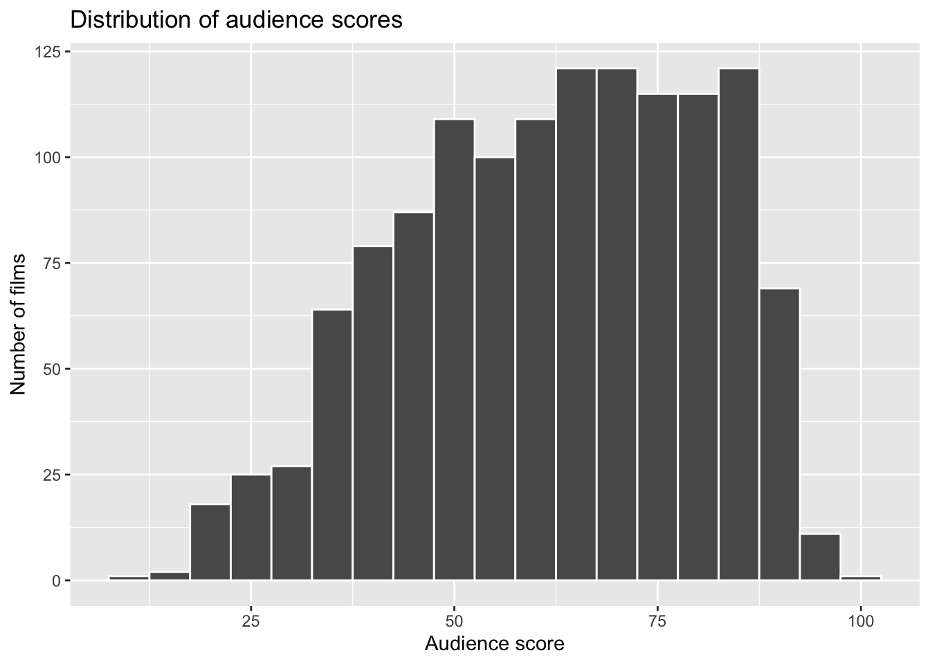
From the histogram and summary statistics, we observe:
The distribution is centred around approximately 60.
The median lies close to this value.
The middle 50% of scores cluster around this central region.
To support this visual inspection, we summarise the variable numerically:
summary(movies$AudienceScore) Min. 1st Qu. Median Mean 3rd Qu. Max.
10.00 49.00 64.00 62.18 77.00 99.00 This suggests that 60 is a reasonable, data-informed point at which to divide films into:
Lower-rated films
Higher-rated films
Importantly:
The cut-off is informed by the observed distribution.
It is chosen before running the hypothesis test.
It is not adjusted to obtain a significant result.
This ensures that the categorisation is statistically justified rather than outcome-driven. We are defining the categories based on the data structure, not on which comparison produces a stronger result.
We use a cut-off of 60 for the following reasons:
The distribution is centred in the low-to-mid 60s.
it produces groups of reasonable size (avoiding very small counts),
it corresponds to an intuitive distinction between
Now that we have justified a reasonable cut-off point based on the observed distribution, we can operationalise “low” and “high” audience reception as a new categorical variable.
a.1) Creating the categorical variable
We now check that both categories contain a sufficient number of films, as extremely small counts can invalidate a Chi-square test.
movies |> count(AudienceScore)# A tibble: 82 × 2
AudienceScore n
<dbl> <int>
1 10 1
2 17 2
3 18 3
4 19 2
5 20 1
6 21 3
7 22 9
8 23 3
9 24 5
10 25 8
# ℹ 72 more rowsmovies <- movies |>
mutate(
AudienceCategory = if_else(AudienceScore < 60, "Low", "High"),
AudienceCategory = factor(AudienceCategory)
)
movies |> count(AudienceCategory)# A tibble: 2 × 2
AudienceCategory n
<fct> <int>
1 High 744
2 Low 551The new variable AudienceCategory is now:
categorical,
has two levels (Low, High),
and is suitable for use in a Chi-square test of independence.
Key idea
When using a Chi-square test, numeric variables must be converted into categories.
The cut-off point should be:
- clearly stated,
- justified using the data, and
- chosen independently of the test outcome.
b) Selecting the two genres for analysis
The variable Genre contains several categories.
However, our research question focuses on comparing two specific genres: Drama and Comedy.
Why do we restrict the dataset?
A Chi-square test of independence compares distributions across categories.
The number of categories determines the size of the contingency table.
If we include all genres, the table becomes larger and interpretation becomes more complex.
For a clear worked example, a 2 × 2 contingency table allows us to focus on the reasoning rather than computational complexity.
By restricting the analysis to two genres, we:
simplify the structure of the contingency table,
make interpretation more transparent,
ensure that expected frequencies remain sufficiently large.
We now subset the dataset to include only Drama and Comedy:
movies_2x2 <- movies |>
  filter(Genre %in% c("Drama", "Comedy")) |>
  droplevels()

movies_2x2
# A tibble: 577 × 16
Movie LeadStudio RottenTomatoes AudienceScore Genre TheatersOpenWeek
<chr> <chr> <dbl> <dbl> <chr> <dbl>
1 21 Jump Street Sony Pict… 85 82 Come… 3121
2 A Late Quartet Entertain… 76 71 Drama 9
3 A Royal Affair Magnolia … 90 82 Drama 7
4 Albert Nobbs Roadside … 56 47 Drama 245
5 American Reun… Universal… 44 63 Come… 3192
6 Amour Sony Pict… 93 82 Drama 3
7 Anna Karenina Focus Fea… 63 51 Drama 16
8 Barfi! UTV Motio… 86 86 Come… 132
9 Beasts of the… Fox Searc… 86 76 Drama 4
10 Big Miracle Universal… 74 64 Drama 2129
# ℹ 567 more rows
# ℹ 10 more variables: OpeningWeekend <dbl>, BOAvgOpenWeekend <dbl>,
# Budget <dbl>, DomesticGross <dbl>, WorldGross <dbl>, ForeignGross <dbl>,
# Profitability <dbl>, OpenProfit <dbl>, Year <dbl>, AudienceCategory <fct>Before running the Chi-square test, we need to construct a contingency table of observed frequencies.
Why?
A Chi-square test does not use raw rows of data directly.
It compares observed counts in each category combination.
Therefore, we must summarise the data into counts for each Genre × AudienceCategory combination.
We now create a table containing only the two relevant categorical variable
movies_2x2 |>
  count(Genre, AudienceCategory)
# A tibble: 4 × 3
Genre AudienceCategory n
<chr> <fct> <int>
1 Comedy High 80
2 Comedy Low 111
3 Drama High 300
4 Drama Low 86This produces a table of observed frequencies, where each cell represents:
a specific genre (Drama or Comedy), and
a specific rating category (Low or High)
These counts form the basis of the Chi-square test.
Step 4: Hypotheses
For a Chi-square test of independence, hypotheses are stated in terms of association, not differences in means.
We test:
\(H_0 : \text{Genre and audience rating category are independent}\)
\(H_1 : \text{Genre and audience rating category are associated}\)
What does “independent” mean?
If the variables are independent:
the proportion of High-rated films is the same for Drama and Comedy,
the proportion of Low-rated films is the same for Drama and Comedy.
In other words, knowing a film’s genre would give us no information about whether it is likely to be rated High or Low.
In words:
The null hypothesis (\(H_0\)) states that there is no association between film genre and audience rating category in the population.
The alternative hypothesis (\(H_1\)) states that there is an association between film genre and audience rating category in the population.
Step 5: Creating the contingency table
Before we can run the Chi-square test, we must organise the data into a contingency table of observed frequencies.
Why do we need a contingency table?
The Chi-square test does not use raw data rows directly.
It compares:
the observed counts in each category combination
with the expected counts we would see if the variables were independent.
So first, we summarise the data into counts.
observed_matrix <- table(
  movies_2x2$Genre,
  movies_2x2$AudienceCategory
)

observed_matrix
         High Low
  Comedy   80 111
  Drama   300  86
Each cell shows the number of films in a given Genre × AudienceCategory combination.
For example:
The value in the Drama–High cell tells us how many Drama films received a High audience rating.
The value in the Comedy–Low cell tells us how many Comedy films received a Low audience rating.
What does this table represent?
This table represents the observed reality in our sample.
In the next step, the Chi-square test will ask:
If genre and rating category were truly independent in the population, would we expect counts like these.
If the observed counts differ substantially from the expected counts under independence, that provides evidence against \(H_0\).
Step 7: Visualisation
Before running the statistical test, it is good practice to inspect the data visually.
A grouped bar chart helps us examine the pattern of counts across categories.
ggplot(movies_2x2, aes(x = Genre, fill = AudienceCategory)) +
  geom_bar(position = "dodge") +
  labs(
    x = "Film genre",
    y = "Number of films",
    fill = "Audience rating category",
    title = "Audience rating category by film genre"
  )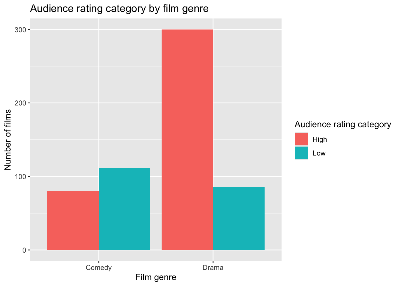
Why do we visualise first?
The plot allows us to:
see whether the distribution of ratings appears different across genres,
check for obvious patterns,
detect any extreme imbalances or data issues.
However:
This plot is descriptive only.
The hypothesis test determines whether the observed pattern is likely to exist in the population.
Visual inspection can suggest a difference, but it cannot tell us whether the difference is statistically significant.
Interpreting counts and percentages
The bar chart above shows counts (frequencies), and the Chi-square test must always be performed using counts.
Why counts are required
The Chi-square statistic compares:
Observed counts
with Expected counts under independence
Percentages cannot be used directly in the formula because the test is based on frequencies.
| Genre | High | Low |
|---|---|---|
| Comedy | 80 | 111 |
| Drama | 300 | 86 |
At first glance, students might focus on the fact that Drama has 300 High-rated films, and conclude that Drama is simply “better”.
But Drama also has many more films overall than Comedy.
To make a fair comparison, we need to compare within each genre.
Raw counts reflect both:
the proportion within a category, and
the total size of that category.
To make a fair comparison, we must compare within each genre.
Why percentages help
Percentages allow us to compare proportions within each genre, removing the effect of different total sizes.
For interpretation, we calculate row percentages (percentages within each genre):
prop.table(observed_matrix, margin = 1)
              High       Low
  Comedy 0.4188482 0.5811518
  Drama  0.7772021 0.2227979
To express these as percentages:
round(prop.table(observed_matrix, margin = 1) * 100, 1)
         High  Low
  Comedy 41.9 58.1
  Drama  77.7 22.3
Now the comparison is clearer:
About 78% of Drama films are rated High
About 42% of Comedy films are rated High
This is much more informative than comparing raw counts alone.
Step 7. b) Plotting the percentages
library(dplyr)

movies_percent <- movies_2x2 |>
  count(Genre, AudienceCategory) |>
  group_by(Genre) |>
  mutate(
    prop = n / sum(n),
    percent = round(prop * 100, 1)
  )
movies_percent
# A tibble: 4 × 5
# Groups: Genre [2]
Genre AudienceCategory n prop percent
<chr> <fct> <int> <dbl> <dbl>
1 Comedy High 80 0.419 41.9
2 Comedy Low 111 0.581 58.1
3 Drama High 300 0.777 77.7
4 Drama Low 86 0.223 22.3This creates:
n(counts)prop(proportion within genre)percent(percentage within genre)
Stacked percentage bar chart with labels
ggplot(movies_percent, aes(x = Genre, y = prop, fill = AudienceCategory)) +
  geom_col() +
  geom_text(aes(label = paste0(percent, "%")),
            position = position_stack(vjust = 0.5),
            colour = "white",
            size = 4) +
  scale_y_continuous(labels = scales::percent_format()) +
  labs(
    x = "Film genre",
    y = "Percentage within genre",
    fill = "Audience rating category",
    title = "Distribution of audience rating category within each genre"
  )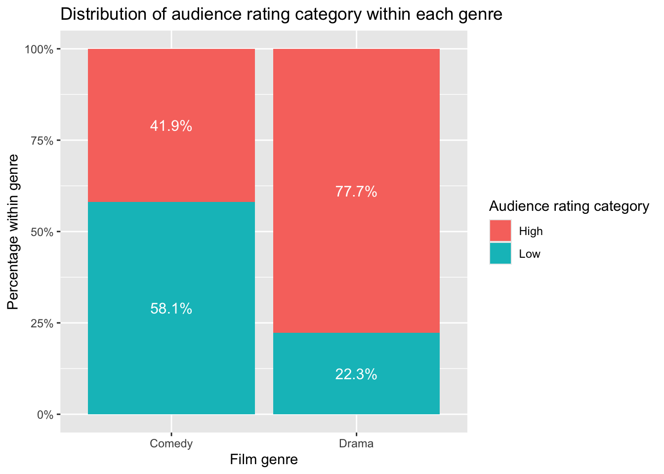
Improve category order (High on top)
Right now “Low” is on top because of factor order.
For interpretation, it is usually clearer to show:
High at the top
Low at the bottom
You can control this explicitly:
movies_percent$AudienceCategory <- factor(
  movies_percent$AudienceCategory,
  levels = c("Low", "High")
)

ggplot(movies_percent,
       aes(x = Genre,
           y = prop,
           fill = AudienceCategory)) +

  geom_col(position = position_stack(reverse = TRUE)) +

  geom_text(
    aes(label = paste0(percent, "%")),
    position = position_stack(vjust = 0.5, reverse = TRUE),
    colour = "white",
    size = 4
  ) +

  scale_y_continuous(
    labels = scales::percent_format()
  ) +

  labs(
    x = "Film genre",
    y = "Percentage within genre",
    fill = "Audience rating category",
    title = "Distribution of audience rating category within each genre"
  )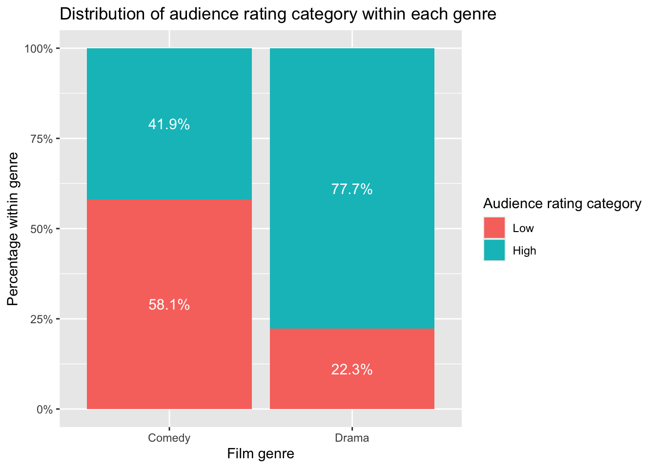
1. Converts AudienceCategory into a factor (categorical variable). This ensures that R treats "Low" and "High" as categories rather than plain text.
2. Specifies the order of the categories. By setting levels = c("Low", "High"), we control how the categories are stacked in the plot. Because stacked bars build from bottom to top, "Low" appears at the bottom and "High" at the top.
3. Supplies the dataset movies_percent to ggplot(). All variables used in the plot must come from this dataset.
4. Defines how variables are mapped to the plot: x = Genre places genre on the horizontal axis. y = prop uses the proportion (within each genre) on the vertical axis. fill = AudienceCategory colours the bars by rating category.
5. Draws stacked bars using the percentage values.geom_col() creates bars from the values stored in prop. position_stack(reverse = TRUE) ensures the stacking order matches the factor order.
6. Adds percentage labels inside each bar segment. paste0(percent, "%") adds a percent sign to each value.vjust = 0.5 centres the label vertically inside each section.colour = "white" improves readability.
7. Formats the vertical axis to display percentages instead of proportions. For example, 0.42 is shown as 42%.
8. Adds clear axis labels, a legend title, and a descriptive plot title. Good labelling improves clarity and communication.
Step 8: Conducting the Chi-square test in R
The Chi-square test works by comparing our observed contingency table to the expected table we would get if the variables were independent.
chi_out <- chisq.test(observed_matrix)
chi_out
    Pearson's Chi-squared test with Yates' continuity correction

data:  observed_matrix
X-squared = 71.389, df = 1, p-value < 2.2e-16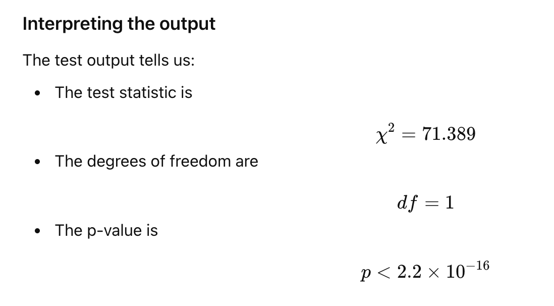
Tip
How to get p-value has a number (not in scientific notation)?
format(chi_out$p.value, scientific = FALSE)[1] "0.00000000000000002932368"Step 9: Effect size (Cramer’s V)
library(rcompanion)

cramer_v <- cramerV(observed_matrix)
cramer_v
Cramer V
0.3556 You:
identify Cramér’s V as the appropriate effect size for Chi-square tests,
give interpretation guidelines (small / moderate / large),
explicitly distinguish effect size from statistical significance.
Step 10: Interpretation
The research question asked whether film genre (Comedy vs Drama) is associated with audience rating category (Low vs High).To address this question, we conducted a Chi-square test of independence, testing the null hypothesis that genre and rating category are independent against the alternative hypothesis that they are associated.
Inspection of the contingency table and the percentage bar plot suggested that the distribution of audience rating categories differs between Comedy and Drama films. In particular, a much larger proportion of Drama films were rated “High” compared with Comedy films.
The Chi-square test showed a statistically significant association between film genre and audience rating category, \(\chi^2(1) = 71.39, , p < .001\). Because the p-value is smaller than the chosen significance level (\(\alpha = 0.05\)), we reject \(H_0\). This provides statistical evidence that film genre and audience rating category are associated in the population.
To assess the strength of this association, we calculated Cramér’s \(V\), which was \(V = 0.36\). According to common guidelines, this represents a moderate association. This indicates that although genre and rating category are related, the relationship is not perfect and there is still variation within each genre.
Importantly, this result is purely statistical and does not imply that genre causes higher or lower audience ratings.