Categorical Data – MSDA IFP

Week 09 – Tutorial 02

1. Tasks for today

This week’s task is highlighted in bold below. Please only focus on completing that task this week. In the next section, you will also find guided sub-steps you may want to consider to complete this week’s task.

Read the College dataset into R, inspect it, and write a concise introduction to the data and its structure.

2) Identify, display, and describe the categorical variables.

Display and describe a selection of numeric variables.

Display and describe at least one relationship between two or three variables.

Finish the report write-up, knit to PDF, and submit.

This tutorial is designed to help you complete Task 2.

1.1 Task 2 – sub-tasks

Tip

Tip: Hover over the footnotes for hints showing useful R functions.

This week you will focus on Task 2: Identify, display, and describe the categorical variables.
Below are some guided sub-steps you may want to consider to complete Task 2.

Reopen last week’s .qmd file, as you will continue last week’s work and build on it.¹

Read the CollegeScores dataset into R (from the provided CSV file in datasets/) and give the object a sensible name, for example college.²
Use functions such as glimpse() or str() to inspect the structure of the dataset and identify which variables are categorical.³
Separate the categorical variables into:
- nominal variables (no natural order), such as State, Control, Region, Locale, and Main
- ordinal variables (meaningful order), such as Selectivity
Convert these categorical variables to factors in R so that they are treated correctly in plots and summaries.⁴
Create frequency tables for at least three categorical variables, showing:
- the count
- the percentage of institutions in each category.⁵
Create bar charts for at least three categorical variables
(for example: number of institutions by Region, by Control, and by Locale).⁶
Improve the readability of your bar charts by:
- rotating x-axis labels if the names are long
- ordering nominal categories by frequency using fct_infreq() where appropriate
- keeping ordinal variables in their natural order
- adding clear axis labels and an informative title with labs().⁷
For one ordinal categorical variable (Selectivity), go further and calculate:
- the median
- the quartiles
- the interquartile range (IQR)
In your written Analysis section, describe the distributions in words. For example:
- Which categories are most common?
- Are some categories rare?
- Is the distribution fairly balanced or dominated by one or two groups?
- For Selectivity, what do the median and IQR tell you?
For each categorical variable in your report, include either the bar plot or the frequency table (not both) to avoid duplicating information.

You do not need to include R output in the report; you only need the written description. Keep this paragraph; you will re-use it in your report.

Data

CollegeScores Dataset

You will work with the CollegeScores dataset in this tutorial.
The dataset includes variables describing each institution’s location, sector, admissions selectivity, tuition costs, enrolment, and the demographic composition of their student body.

You can download the dataset “CollegeScores_teaching_with_selectivity.csv” on Learn ,”Materials - Week 9”

Variable Name	Description
ID	Institution ID number
Name	Name of the institution
State	State where the institution is located
Main	Main campus? (1 = yes, 0 = branch campus)
Control	Control of institution (Private, Profit, Public)
Region	Region of the country (Midwest, Northeast, Southeast, Territory, West)
Locale	Locale of the institution (City, Rural, Suburb, Town)
Enrollment	Undergraduate enrolment
PartTime	Percent of undergraduates who are part-time students
TuitionIn	In-state tuition and fees
TuitionOut	Out-of-state tuition and fees
White	Percent of undergraduates who report being white
Black	Percent of undergraduates who report being black
Hispanic	Percent of undergraduates who report being Hispanic
Asian	Percent of undergraduates who report being Asian
Other	Percent of undergraduates who do not report one of the above categories
AdmitRate	Admission rate
Selectivity	Ordinal category based on admission rate (Highly selective, Moderately selective, Less selective)

2 Worked Example

Consider the dataset provided in datasets/HollywoodMovies.csv, containing 1295 observations on the following 15 variables:

Variable Name	Description
Movie	Title of the movie
LeadStudio	Primary U.S. distributor
RottenTomatoes	Critics' rating (Rotten Tomatoes)
AudienceScore	Audience rating (Rotten Tomatoes)
Genre	Film genre (e.g., Action Adventure, Comedy, Thriller)
TheatersOpenWeek	Number of screens on opening weekend
OpeningWeekend	Opening weekend gross (in millions)
BOAvgOpenWeekend	Average box office income per theatre, opening weekend
Budget	Production budget (in millions)
DomesticGross	U.S. gross income (in millions)
ForeignGross	Foreign gross income (in millions)
WorldGross	Worldwide gross income (in millions)
Profitability	Worldwide gross as a percentage of budget
OpenProfit	Percentage of budget recovered on opening weekend
Year	Year of release

These data were compiled from Box Office Mojo, The Numbers, and Rotten Tomatoes.

We load the tidyverse package as we will use the functions
read_csv() and glimpse() from this package.

Load tidyverse and import the data

library(tidyverse)

read_csv() reads CSV (comma-separated values) files.
The loaded data are stored in an object called movies using the arrow <-.

2.1 Load tidyverse and import the data

movies <- read_csv("HollywoodMovies.csv")

2.2 Inspect the structure of the dataset

glimpse(movies)

Rows: 1,295
Columns: 15
$ Movie            <chr> "2016: Obama's America", "21 Jump Street", "A Late Qu…
$ LeadStudio       <chr> "Rocky Mountain Pictures", "Sony Pictures Releasing",…
$ RottenTomatoes   <dbl> 26, 85, 76, 90, 35, 27, 91, 56, 11, 44, 93, 63, 87, 9…
$ AudienceScore    <dbl> 73, 82, 71, 82, 51, 72, 62, 47, 47, 63, 82, 51, 63, 9…
$ Genre            <chr> "Documentary", "Comedy", "Drama", "Drama", "Horror", …
$ TheatersOpenWeek <dbl> 1, 3121, 9, 7, 3108, 3039, 132, 245, 2539, 3192, 3, 1…
$ OpeningWeekend   <dbl> 0.03, 36.30, 0.08, 0.04, 16.31, 24.48, 1.14, 0.70, 11…
$ BOAvgOpenWeekend <dbl> 30000, 11631, 8889, 5714, 5248, 8055, 8636, 2857, 449…
$ Budget           <dbl> 3.0, 42.0, NA, NA, 68.0, 12.0, NA, 7.5, 35.0, 50.0, 1…
$ DomesticGross    <dbl> 33.35, 138.45, 1.56, 1.55, 37.52, 70.01, 1.99, 3.01, …
$ WorldGross       <dbl> 33.35, 202.81, 6.30, 7.60, 137.49, 82.50, 3.59, 8.54,…
$ ForeignGross     <dbl> 0.00, 64.36, 4.74, 6.05, 99.97, 12.49, 1.60, 5.53, 9.…
$ Profitability    <dbl> 1334.00, 482.88, NA, NA, 202.19, 687.50, NA, 113.87, …
$ OpenProfit       <dbl> 1.20, 86.43, NA, NA, 23.99, 204.00, NA, 9.33, 32.57, …
$ Year             <dbl> 2012, 2012, 2012, 2012, 2012, 2012, 2012, 2012, 2012,…

This helps us identify which variables are categorical and how R is currently storing them.

2.3 Identify categorical variables

Some variables in this dataset are categorical.

a. Nominal categorical variables

LeadStudio
Genre
These have no natural order.

b. Ordinal categorical variable

Year

Although Year is stored as a number, in this worked example we will treat it as an ordered categorical variable because the years follow a meaningful order.

Important

Movie is an identifier variable, not a useful categorical variable for summary plots or frequency tables.

Each movie title appears only once, so plotting Movie would not help us describe the data.

2.4 Convert categorical variables to factors

movies <- movies |>
  mutate(
    LeadStudio = factor(LeadStudio),
    Genre = factor(Genre))

We need the variable Year to be ordered.

first we check the current levels of the variable

levels(movies$Year)

NULL

We also check that R is reading the variable as a factor and not as a character:

class(movies$Year)

[1] "numeric"

to make sure the variable Year is a factor and is order :

movies <- movies |>
  mutate(
    Year = factor(Year, levels = sort(unique(Year)), ordered = TRUE)
  )

Functions:

unique() → find categories
sort() → order them
levels = → tell R the correct order

so, levels = sort(unique(Year)) means “take all the different years in the dataset, sort them from smallest to largest, and use that as the correct order of categories”.

unique(Year)

→ finds all the distinct year values in the dataset

(removes duplicates)
sort(...)

→ arranges those values in increasing order

(e.g. 2008, 2009, 2010, …)
levels = ...

→ tells R:

“these are the categories, and this is their correct order”
ordered = TRUE

tells R that the order matters, so Year is treated as an ordinal variable rather than a nominal one

3 Nominal categorical variables

For nominal variables, we focus on:

frequencies
percentages
bar charts
the most common category (the mode)

We do not calculate the median or IQR for nominal variables.

3.1 Frequency table: `Genre`

tbl_genre <- movies |>
  count(Genre, name = "n") |>
  mutate(
    Percent = round((n / sum(n)) * 100, 1)
  ) |>
  arrange(desc(n))

tbl_genre

# A tibble: 12 × 3
   Genre               n Percent
   <fct>           <int>   <dbl>
 1 Drama             386    29.8
 2 Comedy            191    14.7
 3 Action            170    13.1
 4 Adventure         164    12.7
 5 Thriller          155    12  
 6 Horror             85     6.6
 7 Romantic Comedy    49     3.8
 8 Documentary        41     3.2
 9 Black Comedy       22     1.7
10 Musical            18     1.4
11 Western            10     0.8
12 Concert             4     0.3

3.2 Bar chart: `Genre`

plot_genre <- ggplot(movies, aes(x = Genre)) +
  geom_bar() +
  labs(x = "Movie Genre", y = "Frequency") +
  theme(axis.text.x = element_text(angle = 45, vjust = 1, hjust = 1))
plot_genre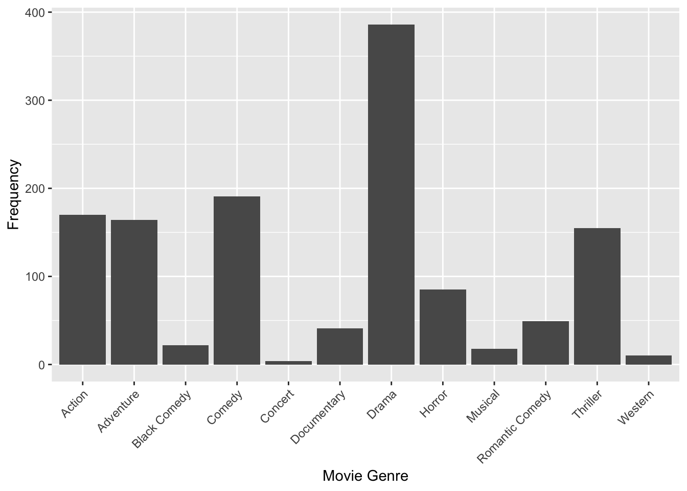

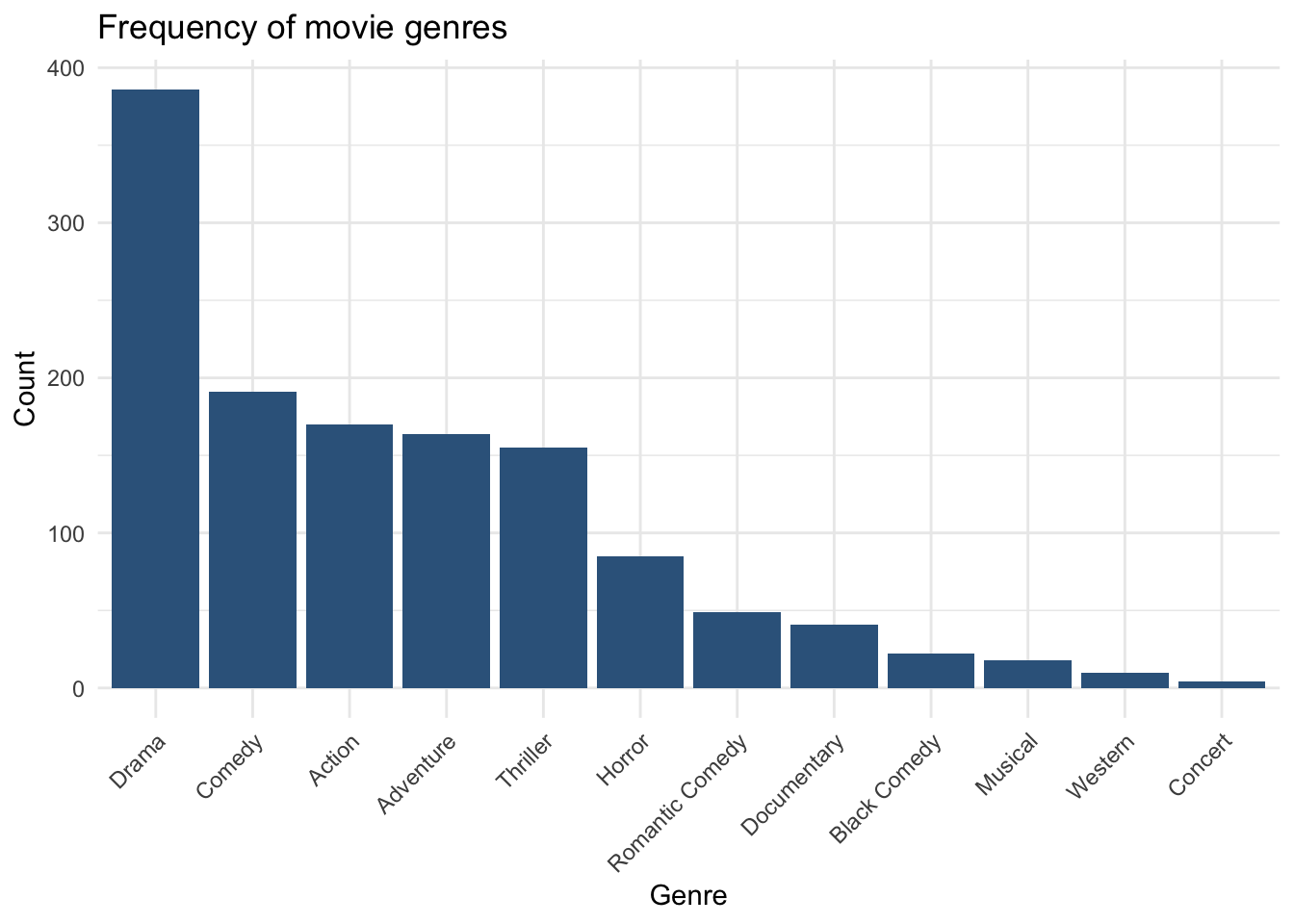
ggplot(movies, aes(x = fct_infreq(Genre))) +
  geom_bar(fill = "steelblue4") +
  labs(
    x = "Genre",
    y = "Count",
    title = "Frequency of movie genres"
  ) +
  theme_minimal() +
  theme(
    axis.text.x = element_text(angle = 45, hjust = 1)
  )

3.3 Frequency table: LeadStudio

tbl_studio <- movies |>
  count(LeadStudio, name = "n") |>
  mutate(
    Percent = round((n / sum(n)) * 100, 1)
  ) |>
  arrange(desc(n))

tbl_studio

# A tibble: 99 × 3
   LeadStudio                              n Percent
   <fct>                               <int>   <dbl>
 1 Warner Bros.                          136    10.5
 2 Universal Pictures                    114     8.8
 3 Lionsgate                             106     8.2
 4 Twentieth Century Fox                 103     8  
 5 Paramount Pictures                     76     5.9
 6 Sony Pictures Releasing                72     5.6
 7 Walt Disney Studios Motion Pictures    72     5.6
 8 Focus Features                         46     3.6
 9 Sony Pictures Classics                 44     3.4
10 Fox Searchlight Pictures               42     3.2
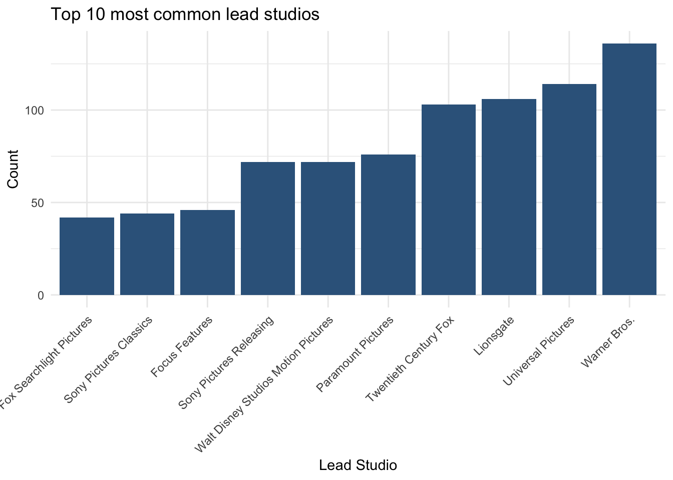
# ℹ 89 more rows

Because there are many studios, it is often clearer to show only the most common ones.

tbl_studio_top10 <- tbl_studio |>
  slice_head(n = 10)

tbl_studio_top10

# A tibble: 10 × 3
   LeadStudio                              n Percent
   <fct>                               <int>   <dbl>
 1 Warner Bros.                          136    10.5
 2 Universal Pictures                    114     8.8
 3 Lionsgate                             106     8.2
 4 Twentieth Century Fox                 103     8  
 5 Paramount Pictures                     76     5.9
 6 Sony Pictures Releasing                72     5.6
 7 Walt Disney Studios Motion Pictures    72     5.6
 8 Focus Features                         46     3.6
 9 Sony Pictures Classics                 44     3.4
10 Fox Searchlight Pictures               42     3.2

3.4 Bar chart: LeadStudio

library(tidyverse)
library(forcats)

plot_LeadStudio  <- ggplot(movies, aes(x = fct_infreq(LeadStudio))) +
  geom_bar() +
  labs(
    x = "Lead Studio (sorted by frequency)",
    y = "Count",
    title = "Frequency of Lead Studios"
  ) +
  scale_y_continuous(
    breaks = seq(0, 150, by = 20)   # More detailed count axis
  ) +
  theme_minimal() +
  theme(
    axis.text.x = element_text(
      angle = 45,
      hjust = 1,
      size = 6,                    # Smaller labels so they fit
      lineheight = 0.8
    ),
    plot.title = element_text(size = 14, face = "bold"),
    axis.text.y = element_text(size = 9)
  )

plot_LeadStudio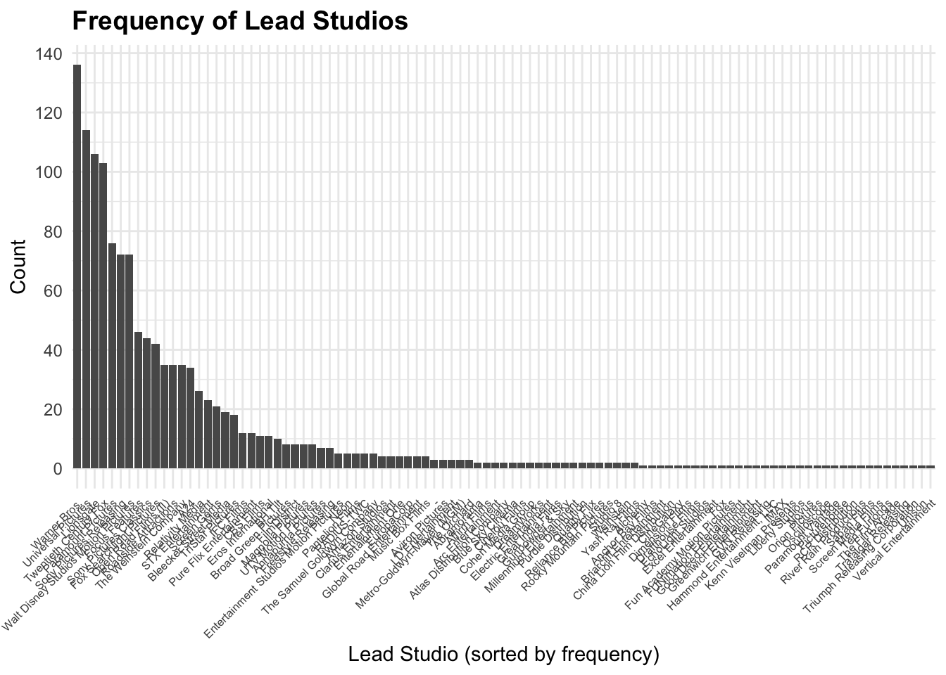

Flip

ggplot(movies, aes(x = fct_infreq(LeadStudio))) +
  geom_bar() +
  coord_flip() +
  labs(x = "Lead Studio (sorted by frequency)", y = "Count") +
  theme_minimal() +
  scale_y_continuous(breaks = seq(0, 150, by = 10))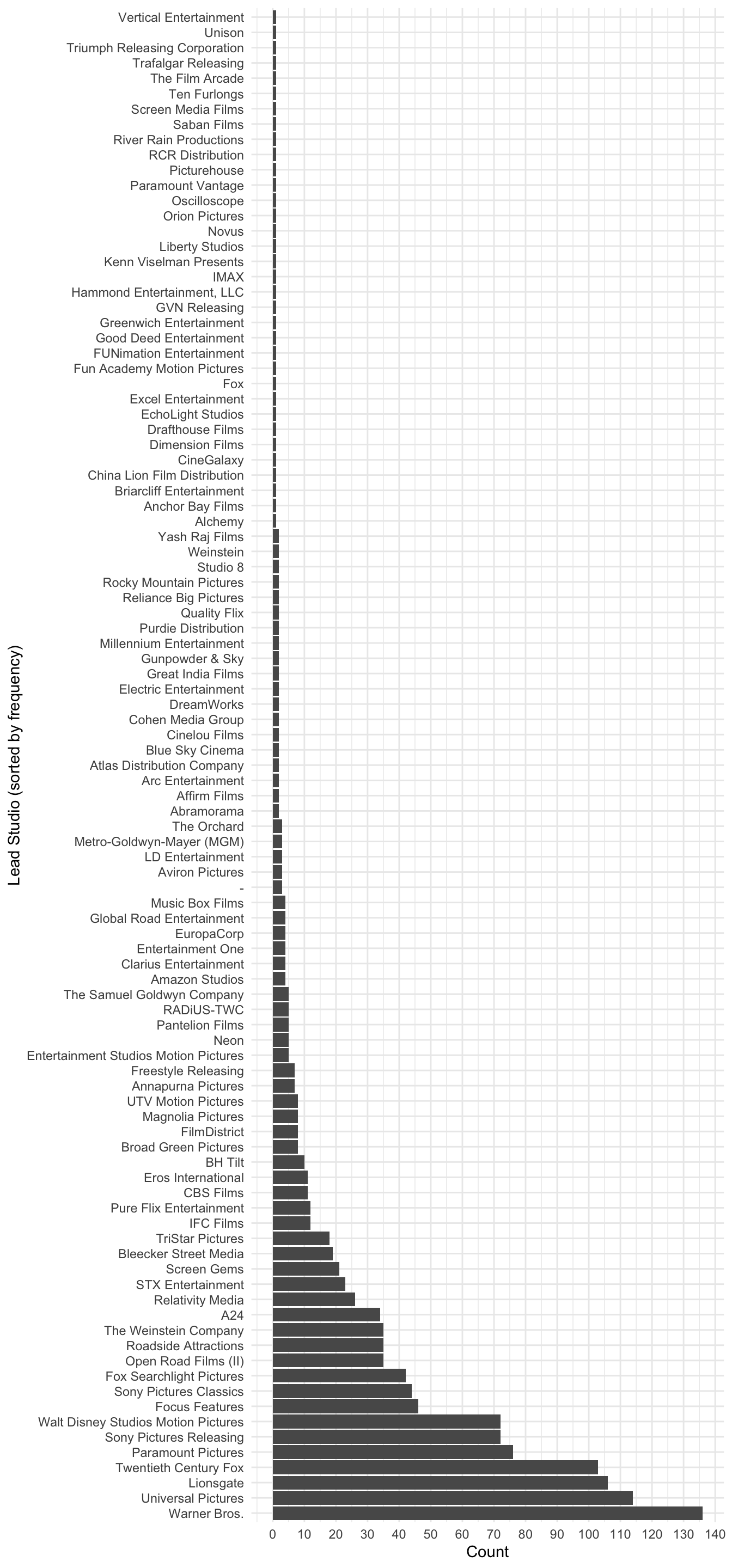

ggplot(tbl_studio_top10, aes(x = fct_reorder(LeadStudio, n), y = n)) +
  geom_col(fill = "steelblue4") +
  labs(
    x = "Lead Studio",
    y = "Count",
    title = "Top 10 most common lead studios"
  ) +
  theme_minimal() +
  theme(
    axis.text.x = element_text(angle = 45, hjust = 1)
  )

3.5 What is the most common category?

For nominal variables, the most common category is the mode.

a. Most common Genre

slice_max(tbl_genre, n, n = 1)

# A tibble: 1 × 3
  Genre     n Percent
  <fct> <int>   <dbl>
1 Drama   386    29.8

This returns the genre with the highest number of movies.

b. Most common Lead Studio

slice_max(tbl_studio, n, n = 1)

# A tibble: 1 × 3
  LeadStudio       n Percent
  <fct>        <int>   <dbl>
1 Warner Bros.   136    10.5

This returns the studio that appears most frequently in the dataset.

What does `slice_max()` do?

n → the column containing the counts
n = 1 → return only the top category

So this code means:

“Give me the category with the highest count.”

How to describe this in your report

For example:

The most common genre in the dataset is Drama, accounting for 29.8% of all movies. This indicates that drama films are the most frequently represented category in the dataset. Similarly, the most common lead studio is Warner Bros., representing 10.5% of the observations. This suggests that this studio appears most frequently in the dataset.

3.6 Ordinal categorical variable: Year

Unlike Genre and LeadStudio, the variable Year has a natural order (time), so it is treated as an ordinal categorical variable.

This means:

the order of categories matters
we can summarise it using median and spread (IQR), not just counts

3.6.1 Frequency distribution of Year

tbl_year <- movies |>
  count(Year, name = "n") |>
  mutate(
    Percent = round((n / sum(n)) * 100, 2)
  )

tbl_year

# A tibble: 7 × 3
  Year      n Percent
  <ord> <int>   <dbl>
1 2012    169    13.0
2 2013    172    13.3
3 2014    197    15.2
4 2015    190    14.7
5 2016    196    15.1
6 2017    182    14.0
7 2018    189    14.6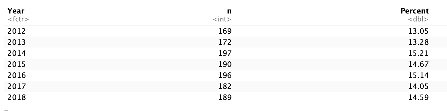

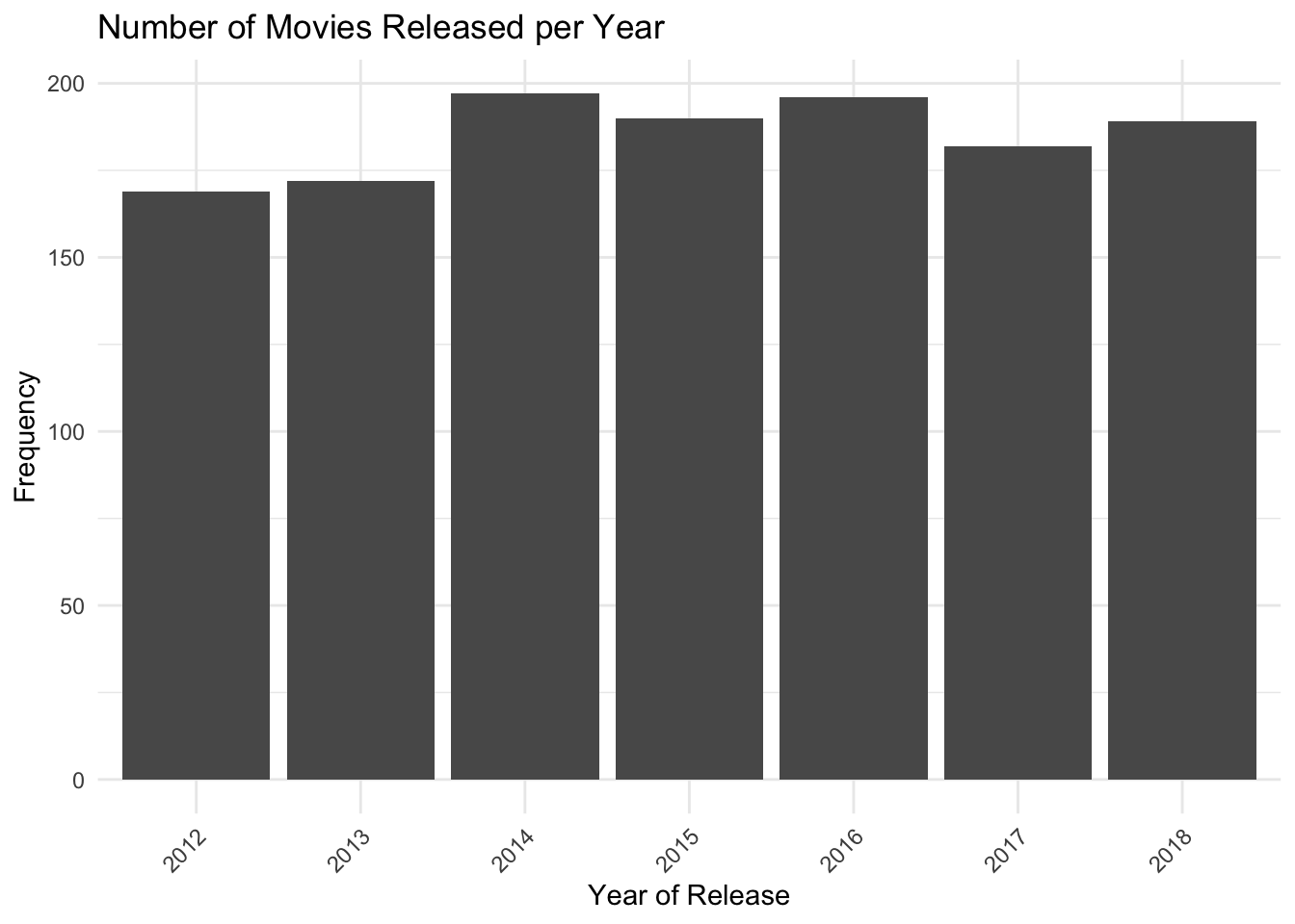
This shows how many movies were released in each year.

Year frequency plot

ggplot(movies, aes(x = factor(Year))) +
geom_bar() +
labs(
x = "Year of Release",
y = "Frequency",
title = "Number of Movies Released per Year"
) +
theme_minimal() +
theme(
axis.text.x = element_text(
angle = 45,
hjust = 1
)
)

Formatting tables nicely

library(kableExtra)


Attaching package: 'kableExtra'

The following object is masked from 'package:dplyr':

    group_rows

kbl(
  list(
    tbl_genre,
    tbl_studio_top10
  ),
  booktabs = TRUE,
  digits = 2,
  col.names = c("Category", "Count", "Percent")
)

Category	Count	Percent
Drama	386	29.8
Comedy	191	14.7
Action	170	13.1
Adventure	164	12.7
Thriller	155	12.0
Horror	85	6.6
Romantic Comedy	49	3.8
Documentary	41	3.2
Black Comedy	22	1.7
Musical	18	1.4
Western	10	0.8
Concert	4	0.3

Category	Count	Percent
Warner Bros.	136	10.5
Universal Pictures	114	8.8
Lionsgate	106	8.2
Twentieth Century Fox	103	8.0
Paramount Pictures	76	5.9
Sony Pictures Releasing	72	5.6
Walt Disney Studios Motion Pictures	72	5.6
Focus Features	46	3.6
Sony Pictures Classics	44	3.4
Fox Searchlight Pictures	42	3.2

If you prefer separate tables with captions you can reference in the text:

# Genre table
tbl_genre |>
  kbl(
    booktabs = TRUE,
    digits = 2,
    caption = "Frequency distribution of movie genres",
    col.names = c("Genre", "Count", "Percent")
  )

Frequency distribution of movie genres
Genre	Count	Percent
Drama	386	29.8
Comedy	191	14.7
Action	170	13.1
Adventure	164	12.7
Thriller	155	12.0
Horror	85	6.6
Romantic Comedy	49	3.8
Documentary	41	3.2
Black Comedy	22	1.7
Musical	18	1.4
Western	10	0.8
Concert	4	0.3

# Lead studio table (top 10)
tbl_studio_top10 |>
  kbl(
    booktabs = TRUE,
    digits = 2,
    caption = "Top 10 most common lead studios",
    col.names = c("Lead Studio", "Count", "Percent")
  )

Top 10 most common lead studios
Lead Studio	Count	Percent
Warner Bros.	136	10.5
Universal Pictures	114	8.8
Lionsgate	106	8.2
Twentieth Century Fox	103	8.0
Paramount Pictures	76	5.9
Sony Pictures Releasing	72	5.6
Walt Disney Studios Motion Pictures	72	5.6
Focus Features	46	3.6
Sony Pictures Classics	44	3.4
Fox Searchlight Pictures	42	3.2

Then in your .qmd text you can reference them like:

Table \@ref(tab:genre-table) shows the frequency and percentage of each film genre.

Table \@ref(tab:studio-table) summarises the ten most common lead studios.

(using the corresponding chunk labels, e.g. {r genre-table} and {r studio-table} for the chunks that create each kbl).

What is the most common category?

Most common genre = category with the highest frequency
Most common lead studio = category with the highest frequency

You can identify this from the sorted tables or by using slice_max():

slice_max(tbl_genre, n, n = 1)

# A tibble: 1 × 3
  Genre     n Percent
  <fct> <int>   <dbl>
1 Drama   386    29.8

slice_max(tbl_studio, n, n = 1)

# A tibble: 1 × 3
  LeadStudio       n Percent
  <fct>        <int>   <dbl>
1 Warner Bros.   136    10.5

Footnotes

Hint: Open the same .qmd file you used for Task 1 so you keep building a single report.↩︎
Hint: Use read_csv("datasets/CollegeScores_teaching.csv") from the readr package.↩︎
Hint: Try glimpse(college) from dplyr or str(college).↩︎
Hint: Use mutate() with factor(), for example
college <- college |> mutate(Control = factor(Control), Region = factor(Region)).↩︎
Hint: college |> count(Control) |> mutate(Percent = round(n / sum(n) * 100, 2)).↩︎
Hint: Use ggplot(college, aes(x = Control)) + geom_bar().↩︎
Hint: theme(axis.text.x = element_text(angle = 45, hjust = 1)) and fct_infreq() from forcats.↩︎

1. Tasks for today

1.1 Task 2 – sub-tasks

Data

2 Worked Example

Load tidyverse and import the data

2.1 Load tidyverse and import the data

2.2 Inspect the structure of the dataset

2.3 Identify categorical variables

2.4 Convert categorical variables to factors

3 Nominal categorical variables

3.1 Frequency table: Genre

3.2 Bar chart: Genre

3.3 Frequency table: LeadStudio

3.4 Bar chart: LeadStudio

3.5 What is the most common category?

What does slice_max() do?

How to describe this in your report

3.6 Ordinal categorical variable: Year

3.6.1 Frequency distribution of Year

Formatting tables nicely

What is the most common category?

Footnotes

3.1 Frequency table: `Genre`

3.2 Bar chart: `Genre`

What does `slice_max()` do?