| Variable Name | Description |
|---|---|
| Name | Name of the institution |
| State | US state where the institution is located |
| ID | Institution ID number |
| Main | Main campus indicator (1 = main campus, 0 = branch campus) |
| Control | Control of institution (Private, Profit, Public) |
| Region | US region (Midwest, Northeast, Southeast, West, etc.) |
| Locale | Locale type (City, Suburb, Town, Rural) |
| Enrollment | Undergraduate enrolment (number of students) |
| AdmitRate | Admission rate (proportion of applicants admitted) |
| Cost | Average total cost (tuition, room, board, etc.) |
| PartTime | Percent of undergraduates who are part-time students |
| TuitionIn | In-state tuition and fees |
| TuitionOut | Out-of-state tuition and fees |
– MSDA IFP
Week 13 – Tutorial 06 - Correlations
1. Tasks for formative report
This week’s task is highlighted in bold below. Please only focus on completing that task this week. In the next section, you will also find guided sub-steps you may want to consider to complete this week’s task.
- Read the College dataset into R, inspect it, and write a concise introduction to the data and its structure.
- Display and describe the categorical variables.
- Display and describe a selection of numeric variables.
4) Test at least one research question using an appropriate hypothesis test.
- Finish the report write-up, knit to PDF, and submit.
This tutorial is designed to help you complete Task 4.
1.1 Task 4 – sub-tasks
Tip
Tip: Hover over the footnotes for hints showing useful R functions.
This week you will focus on Task 4: Test at least one research question using an appropriate hypothesis test.
Below are guided sub-steps you may want to follow, using the structure required in Assessment Stage 2.
Your required structure for each research question
For each research question, you must complete these steps in order:
- State the research question in your own words.
- Write the null hypothesis (\(H_0\)) and the alternative hypothesis (\(H_1\)).
- Identify the variables involved and their roles (grouping variable, outcome variable).
- Consider which statistical test is appropriate, and justify your choice.
- Prepare the data only as required to answer the research question
(minimal subsetting only where necessary).
- Conduct the statistical analysis in R.
- Report the relevant statistical output
(t, df, p-value, and confidence interval).
- Produce one appropriate visualisation and refer to it in the text.
Your writing should be clear and concise.
Interpretation should be brief and factual.
Data
CollegeScores Dataset
You will work with the CollegeScores dataset in this tutorial.
At the link CollegeScores_teaching.csv you will find information about 400 higher-education institutions in the United States.
The dataset includes variables describing each institution’s location, sector (public/private), tuition costs, enrolment, and the demographic composition of their student body.
Research questions for this tutorial
RQ1: Is undergraduate enrollment associated with in-state tuition?
RQ2: Is the percentage of part-time students associated with in-state tuition?
Each of these involves two numerical variables, so a Pearson correlation test is appropriate.
2 Worked Example
In this worked example, we illustrate the full reasoning process behind a hypothesis test, from a research question to statistical analysis and reporting.
The aim is to show how statistical analysis is driven by a research question, not by R commands.
We use the dataset provided in datasets/HollywoodMovies.csv, which contains information on 1295 films, including their genre and audience ratings.
To make this comparison suitable for a statistical test, we will focus on two genres only.
| Variable Name | Description |
|---|---|
| Movie | Title of the movie |
| LeadStudio | Primary U.S. distributor |
| RottenTomatoes | Critics' rating (Rotten Tomatoes) |
| AudienceScore | Audience rating (Rotten Tomatoes) |
| Genre | Film genre (e.g., Action Adventure, Comedy, Thriller) |
| TheatersOpenWeek | Number of screens on opening weekend |
| OpeningWeekend | Opening weekend gross (in millions) |
| BOAvgOpenWeekend | Average box office income per theatre, opening weekend |
| Budget | Production budget (in millions) |
| DomesticGross | U.S. gross income (in millions) |
| ForeignGross | Foreign gross income (in millions) |
| WorldGross | Worldwide gross income (in millions) |
| Profitability | Worldwide gross as a percentage of budget |
| OpenProfit | Percentage of budget recovered on opening weekend |
| Year | Year of release |
These data were compiled from Box Office Mojo, The Numbers, and Rotten Tomatoes.
2.1 Research context and research question
Film industry analysts are often interested in whether financial investment in a film is related to its financial success.
Research question
Is production budget associated with worldwide gross revenue?
This question concerns a possible relationship between:
Budget(production budget, in millions of dollars)WorldGross(worldwide box office revenue, in millions of dollars)
Both variables are numeric, so a Pearson correlation test is appropriate.
2.3 Step 1 – Visual inspection
Before calculating a correlation, we must inspect a scatterplot.
library(readr)


movies <- read_csv("HollywoodMovies.csv")
Rows: 1295 Columns: 15
── Column specification ────────────────────────────────────────────────────────
Delimiter: ","
chr (3): Movie, LeadStudio, Genre
dbl (12): RottenTomatoes, AudienceScore, TheatersOpenWeek, OpeningWeekend, B...
ℹ Use `spec()` to retrieve the full column specification for this data.
ℹ Specify the column types or set `show_col_types = FALSE` to quiet this message.ggplot(movies, aes(x = Budget, y = WorldGross)) +
geom_point() +
labs(
x = "Production budget (millions)",
y = "Worldwide gross (millions)",
title = "Scatterplot of budget and worldwide gross"
)Warning: Removed 239 rows containing missing values or values outside the scale range
(`geom_point()`).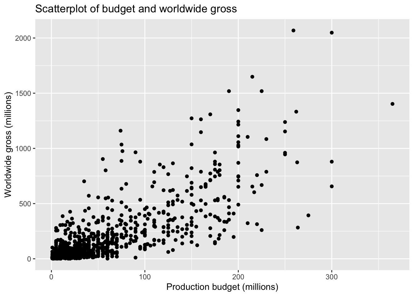
Adding a line of best fit
ggplot(movies, aes(x = Budget, y = WorldGross)) +
  geom_point() +
  geom_smooth(method = "lm", se = FALSE) +
  labs(
    x = "Production budget (millions)",
    y = "Worldwide gross (millions)",
    title = "Budget and worldwide gross with line of best fit"
  )
`geom_smooth()` using formula = 'y ~ x'Warning: Removed 239 rows containing non-finite outside the scale range
(`stat_smooth()`).Warning: Removed 239 rows containing missing values or values outside the scale range
(`geom_point()`).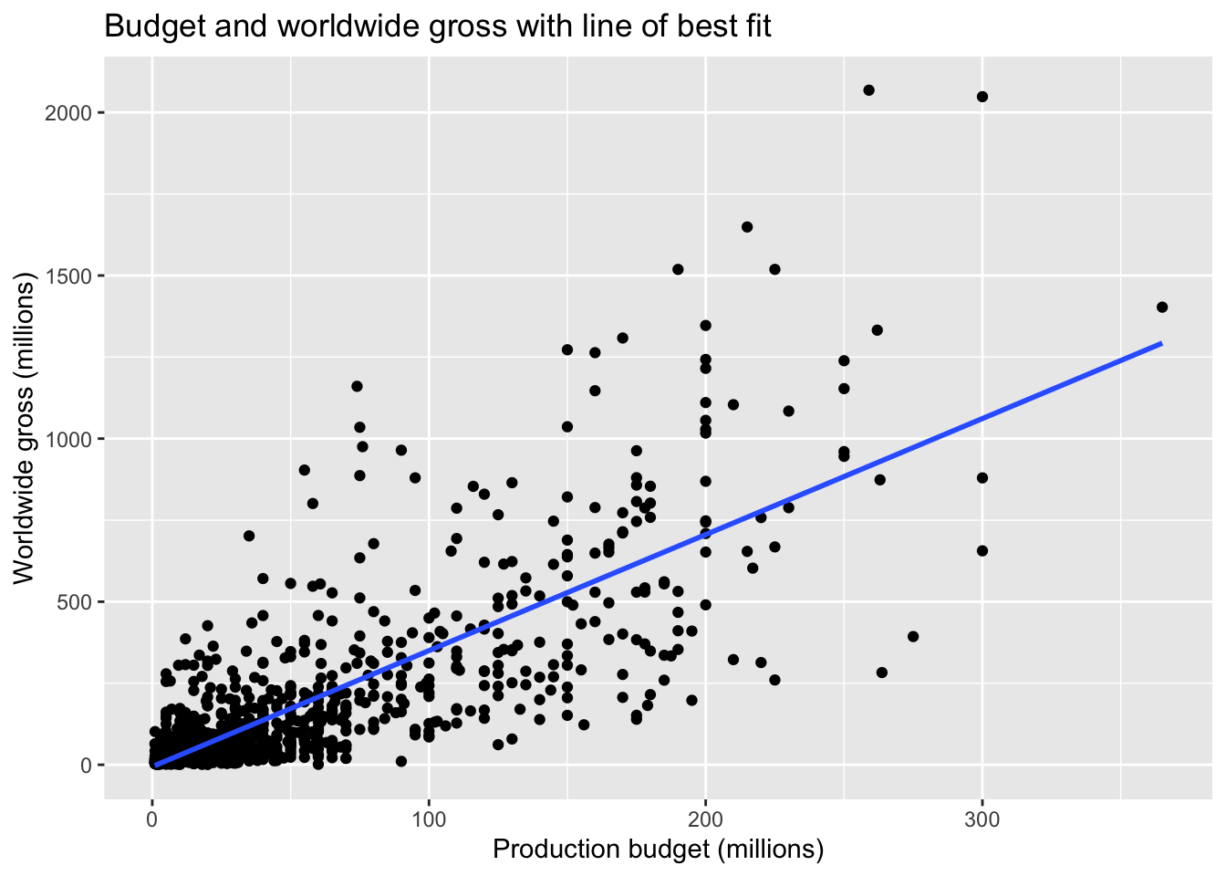
Interpreting the scatterplot (before running the test)
Before calculating the correlation coefficient, we carefully inspect the scatterplot.
When looking at a scatterplot, we ask:
Is there an apparent relationship?
The points appear to trend upwards from left to right, suggesting a possible positive relationship between production budget and worldwide gross.Is the relationship approximately linear?
The overall pattern appears roughly linear, although there is noticeable spread around the line of best fit.Are there outliers?
There are some films with very high budgets and extremely high gross values. These observations may influence the strength of the correlation.How strong does the relationship look visually?
The points are not tightly clustered around the line, but the upward trend is clear. This suggests a moderate to strong positive relationship.
At this stage, we do not draw statistical conclusions.
We are simply describing what the graph suggests.
What can we observe?
From the scatterplot:
Films with larger production budgets tend to have higher worldwide gross.
The relationship appears positive (as budget increases, gross increases).
The pattern is approximately linear.
There is considerable variation — films with similar budgets sometimes have very different gross outcomes.
A small number of high-budget films may influence the overall trend.
This visual inspection suggests that a positive linear relationship may exist, which we can now formally test using Pearson’s correlation.
Step 2: State the hypotheses
For a Pearson correlation test, we test whether the population correlation is equal to zero.
The hypotheses are:
The null hypothesis is \(H_0 : \rho = 0\) , meaning that there is no linear relationship between production budget and worldwide gross in the population.
The alternative hypothesis is \(H_1 : \rho \ne 0\). There is a linear relationship between production budget and worldwide gross in the population.
This is a non-directional (two-sided) test, because we are testing for the presence of a relationship, not specifying whether it is positive or negative.
In words
The null hypothesis (\(H_0\)) states that production budget and worldwide gross are not linearly related in the population.
The alternative hypothesis (\(H_1\)) states that production budget and worldwide gross are linearly related in the population.
Understanding correlation testing
In correlation testing:
We test whether the population correlation (\(\rho\)) differs from zero.
The sample correlation (\(r\)) is our estimate of \(\rho\).
The p-value tells us whether the observed \(r\) is statistically different from zero.
Step 3: Run the correlation test in R
We now calculate the Pearson correlation coefficient and test whether it differs from zero.
cor_test <- cor.test(movies$Budget, movies$WorldGross)
cor_test
    Pearson's product-moment correlation

data:  movies$Budget and movies$WorldGross
t = 40.979, df = 1054, p-value < 2.2e-16
alternative hypothesis: true correlation is not equal to 0
95 percent confidence interval:
 0.7594115 0.8060409
sample estimates:
      cor
0.7838287
From the test output:
\(r = 0.7838287\)
\(p < 2.2 \times 10^{-16}\)
95% CI: \([0.759, 0.806]\)
How to interpret the output (thought process)
When reading the output, follow this order:
1. Direction
Is \(r\) positive or negative?
- If \(r > 0\) → higher budgets tend to be associated with higher worldwide gross.
- If \(r < 0\) → higher budgets tend to be associated with lower worldwide gross.
2. Strength
How large is \(|r|\)?
Use the strength guidelines introduced earlier:
- 0.00–0.19 → very weak
- 0.20–0.39 → weak
- 0.40–0.59 → moderate
- 0.60–0.79 → strong
- 0.80–1.00 → very strong
3. Statistical evidence
Check the \(p\)-value:
- If \(p < 0.05\) → reject \(H_0\)
- If \(p \ge 0.05\) → fail to reject \(H_0\)
Then check the confidence interval:
- If the CI does not include 0 → statistically significant
- If the CI includes 0 → not statistically significant
1. Direction
Is \(r\) positive or negative?
\(r = 0.7838\)
This is positive.
Therefore:
Higher production budgets tend to be associated with higher worldwide gross.
The scatterplot also supports this: the line of best fit slopes upward.
2. Strength
How large is \(|r|\)?
- \(|r| = 0.7838\)
Using the guideline:
0.60–0.79 → strong
0.80–1.00 → very strong
Since 0.7838 is very close to 0.80 but still within 0.60–0.79:
The relationship is strong (very close to very strong).
This indicates a substantial linear association between budget and worldwide gross.
What do the vertical bars \(|r|\) mean?
The vertical bars mean:
Ignore the sign and look only at the magnitude.
Why?
Because strength is about how large the relationship is, not whether it is positive or negative.
For example:
- \(r = 0.75\) → strong
- \(r = -0.75\) → also strong
Both have the same strength because:
\[ |0.75| = |-0.75| = 0.75 \]
So when interpreting strength, we use \(|r|\).
3. Statistical evidence
p-value
\(p < 2.2 \times 10^{-16}\)
This is far smaller than \(\alpha = 0.05\).
Therefore:
We reject \(H_0\).
There is strong statistical evidence that the population correlation is not zero.
Confidence interval
95% CI: \([0.759, 0.806]\)
The interval does not include 0.
Therefore:
The result is statistically significant.
The true population correlation is likely between 0.76 and 0.81.
Step 4: Interpretation
We tested whether production budget is linearly associated with worldwide gross revenue for films.
A Pearson correlation test showed a strong positive linear relationship between production budget and worldwide gross, \(r = 0.784\), 95% CI \([0.759, 0.806]\), \(p < .001\). Because the p-value is smaller than the chosen significance level (\(\alpha = 0.05\)), we reject \(H_0\). This provides statistical evidence of a positive linear association between production budget and worldwide gross in the population. The confidence interval does not include 0, which further supports that the relationship is statistically significant.
In practical terms, films with higher production budgets tend to generate higher worldwide gross revenue.
Importantly, this result describes an association and does not imply that higher budgets cause higher revenue.